import numpy as np
from scipy.stats import norm,uniform,lognorm
import matplotlib.pyplot as plt
import seaborn as sbn
import pandas as pd

np.random.seed(348348756)

plt.style.use('ggplot')

Inference and Monte Carlo Markov Chains

Frequentists are used to the idea of hypothesis tests like

(2)\[\begin{eqnarray} H_0: \mu = 0 \nonumber\\ H_1: \mu \neq 0 \nonumber \end{eqnarray}\]

To proceed, we examine in expecation the moments of a parameter of interest. For example the variance of a mean \(\bar{x}\) is computed as

\[ Var(x) = E_x\left[\left(x - E(x)\right)^2\right] \]

an interesting take on this expecation is that it is with respect to “data”, since the true but unknown mean of \(x\) exists and can be written as \(\mu_x\), making the above

\[ Var(x) = E_x\left[\left(x - \mu_x \right)^2\right] \]

This variance can then be estimated from a sample having \(N\) observations of data using

\[ \hat{Var(x)} = \frac{\sum_{i=1}^N(x_i-\bar{x})^2}{N} \]

where \(\bar{x} = \frac{\sum_{i=1} x_i }{N}\).

From there, confidence intervals, z scores, and other measures can be computed inference.

The frequentist approach typically follows these steps:

1. Collect data

2. Define a model

3. Use data and model to calculate parameters of interest

4. Use parameters to test hypotheses

The Bayesian approach differs a bit

1. Collect data

2. Define a model

3. Use data and model to sample many times from the posterior distribution of parameters of interest (can be multivariate [many parameters])

4. Use the parameter samples to test hypothesis

It is really in steps (3) and (4) that things differ. This notebook shows how this is implemented.

Note

Once can say that inference for a Bayesian is “attaching probabilities to statements”. These statements can be problem driven and need to be as formally defined as the hypothesis test above.

A simple model

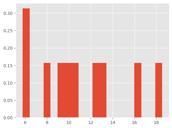
For having something concrete to play with, let’s resurrect our simple example yet again:

data = norm(10,3).rvs(10)
sigma = 3          # Note this is the std of x
mu_prior = 8
sigma_prior = 1.5  # Note this is our prior on the std of mu

plt.hist(data,bins=20, density=True)
plt.show()

and we will again use our simple sampler:

# a fairly basic mh mcmc random walk sampler:
def sampler(data, samples=4, mu_init=9, sigma= 1, proposal_width=3, 
            mu_prior_mu=10, mu_prior_sd=1):
    mu_current = mu_init
    posterior = [mu_current]
    for i in range(samples):
        # suggest new position
        mu_proposal = norm(mu_current, proposal_width).rvs()

        # Compute likelihood by multiplying probabilities of each data point
        likelihood_current = norm(mu_current, sigma).pdf(data).prod()
        likelihood_proposal = norm(mu_proposal, sigma).pdf(data).prod()
        
        # Compute prior probability of current and proposed mu        
        prior_current = norm(mu_prior_mu, mu_prior_sd).pdf(mu_current)
        prior_proposal = norm(mu_prior_mu, mu_prior_sd).pdf(mu_proposal)
        
        p_current = likelihood_current * prior_current
        p_proposal = likelihood_proposal * prior_proposal
        
        # Accept proposal?
        c = np.min((1,p_proposal / p_current))
        
        accept = np.random.rand() <= c
                
        if accept:
            # Update position
            mu_current = mu_proposal
        
        posterior.append(mu_current)
        
    return np.array(posterior)

With that defined, let’s take 5000 samples from the posterior:

chain = sampler(data,samples=5000,mu_init=9,sigma=sigma,proposal_width=3,
                mu_prior_mu=mu_prior,mu_prior_sd = sigma_prior)

Using our chain for inference

In what follows, I assume we have already assessed chain convergence and are satisfied with a burn-in of 100.

In the code below, I ask a number of questions (you might call this inference) using our sampled posterior values, starting with ones most similar to frequentist statistics:

chain_s = chain[100:]

Let’s plot the histogram of our sample mean values:

plt.figure(figsize=(10,8))
plt.hist(chain_s, bins=75, density=True)
plt.show()

Here are some common inference-related questions a frequentist might ask:

print( "The mean is: ", chain_s.mean())
print( "The standard deviation is: ", chain_s.std())
print( "The median is: ", np.percentile(chain_s,50))
print( "The 95% Credible Interval is: ",np.percentile(chain_s,[2.5,97.5]))
print( "The probability that the mean is greater than 10: ", \
            chain_s[chain_s>10].shape[0]/chain_s.shape[0])

The mean is:  10.180621628544616
The standard deviation is:  0.8093876372087345
The median is:  10.196002242838691
The 95% Credible Interval is:  [ 8.51523653 11.77003799]
The probability that the mean is greater than 10:  0.6015098959396041

Some observations:

1. Notice that the MCMC analysis above provides thousands of potential mean estimates. Some of these are closer to the fat part of the posterior while others are not. We take an average of each of these potential mean values to estimate the mean of the posterior. We can also use these potential mean values to compute other moments of interest (like standard deviation).

2. We can also use the sample of means to compute non-parametric credibility intervals. Note this doesn’t make any distributional assumptions over the sample parameter values. For a Bayesian, the credible interval can be interpreted as the probability that the parameter of interest resides in the range given by the interval. For a frequentist confidence interval, it must be interpreted differently:

   Frequentist Confidence Interval

   Suppose we have a 95% confidence interval defined over [2.1, 5.9]. It is not correct to say that there is a 95% chance that the “true” parameter resides within 2.1 and 5.9. Rather one needs to phrase it as follows: If you collected many different data sets and computed your statistic, 95% of these computed statistics would reside in the range 2.1 and 5.9. It is more of a statement about your confidence in the method you are using. Recall, that for a frequentist, the unknown parameter is non-random so that either the parameter resides within 2.1 and 5.9 or not.

3. For “one-sided” hypothesis testing, we can simply compute the fraction of cases above the critical value that is being tested.

In short, samples from the posterior can provide nearly any type of inference related question we might want to ask. Overlaying the credible interval on our histogram of sampled mean values, shows that sample itself reveals what is and isn’t most likely:

plt.figure(figsize=(10,8))
plt.hist(chain_s, density=True, bins=75)
plt.axvline(np.percentile(chain_s,[2.5,97.5])[0], c='k', ls='--')
plt.axvline(np.percentile(chain_s,[2.5,97.5])[1], c='k', ls='--');

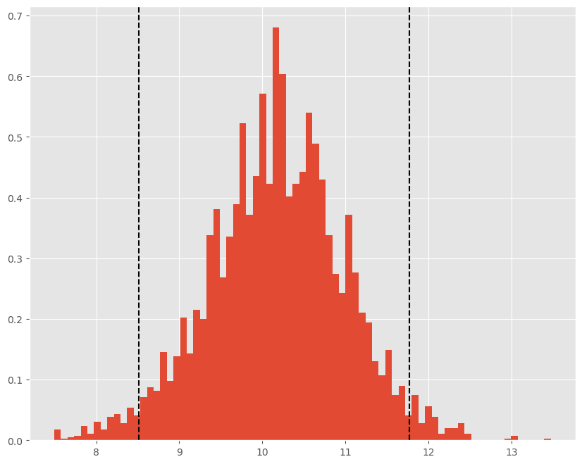
While the last question isn’t one we typically ask in a frequentist setting, we could by imposing normality from our model estimates and calculating areas under the pdf. Alternatively, we could perform a bootstrapping excercise as we did earlier in the class. The posterior pdf pictured above does not assume normality of our parameters and in that way is similar to the bootstrap approach for inference.

The Credible Interval above can be interpreted as

There is a 95% chance that \(\theta\) is in the interval [8.84,9.95]

Note: the numbers in brackets will change depending on the credible interval printed above.

Classical Hypothesis testing

In frequentist statistics, we often perform test as follows:

\[\begin{split} H_0 : \theta = 0 \\ H_1 : \theta \ne 0 \end{split}\]

This isn’t very easy to do in a Bayesian Context. We can see that no values of our chain is exactly equal to 0 and this would likely be the case even if our mean for this problem was centered on zero.

print( "Number of cases where theta=10: ", chain_s[chain_s==10].shape[0])

Number of cases where theta=10:  0

So does this mean we have 100% evidence that theta isn’t 10? A Bayesian would typically recast this question into an interval:

\[\begin{split} H_0 : \theta \in 10 \pm .1 \\ H_1 : \theta \notin 10 \pm .1 \end{split}\]

print( "Probability of H_0: ",chain_s[(chain_s<=10.1) & (chain_s>=9.9)].shape[0] / chain_s.shape[0])

Probability of H_0:  0.09610283615588655

So Bayesians like to attach probabilities to statements. Additionally note that due to our very small sample size, the prior is definitely affecting our inference here.

Highest Posterior Density (HPD) Intervals

For skewed or multimodal posteriors, credible intervals may not be as enlightening as they could be. Suppose we have a MH markov chain and our posterior pdf is plotted below. The HPD interval, sets a minimum probability threshold for parameters (e.g. posterior value must be greater than .025) and examines the interval of values of \(\theta\) that have more than a .025% chance of being observed.

Note

Skewed of multimodel samples from a posterior can be a sign that your chain hasn’t converged or some other underlying pathology with your model.

Consider this skewed chain and an exercise of sliding a horizontal dotted black line down until it’s y-value is equal to the cutoff you as an analyst care about (e.g. .025):

skewed_chain = lognorm(1,8).rvs(10000)

plt.figure(figsize=(10,8))
plt.hist(skewed_chain,bins=100, density=True)
plt.axhline(.025, c='k', linestyle='--')
plt.axvline(12.74, c='k', linestyle='--')
plt.xlabel('$\\theta$')
plt.xlim((7,20))
plt.title('Posterior')
plt.show()

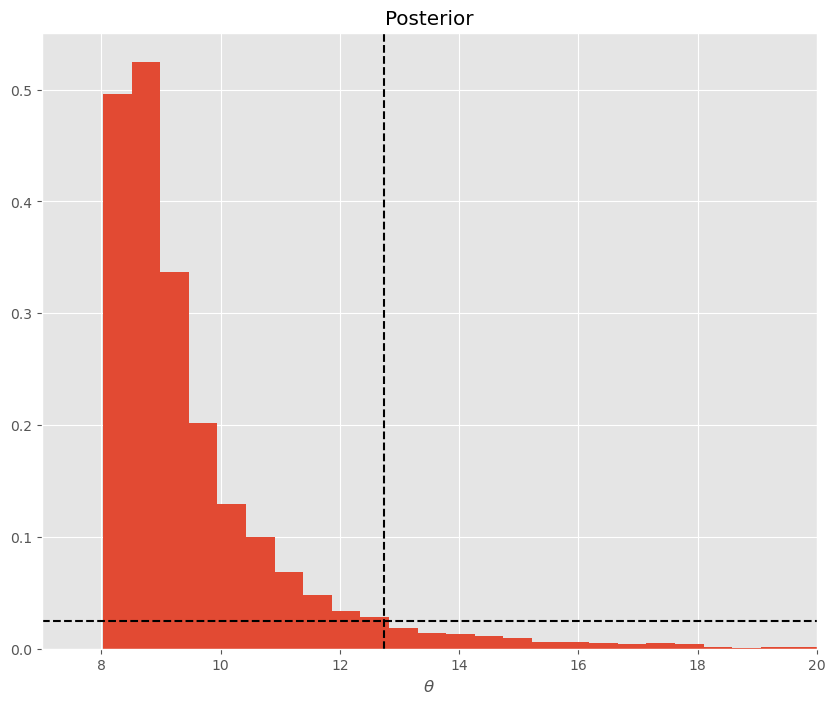
Note on the left hand size of the posterior, there is no region where the occurence of \(\theta\) is less than .025.

print("The mean is: ", skewed_chain.mean())
print("The standard deviation is: ", skewed_chain.std())
print("The median is: ", np.percentile(skewed_chain,50))
print("The 95% Credible Interval is: ",np.percentile(skewed_chain,[2.5,97.5]))

The mean is:  9.643799028459755
The standard deviation is:  2.1150266705678
The median is:  9.011681077018235
The 95% Credible Interval is:  [ 8.15066093 15.03739996]

Note the credible interval here is a bit strange, as there is large probability mass, near the minimum observed value. So turning to the HPD interval:

print("The highest posterior density interval is (approximately): ")
print("["+str(skewed_chain.min())+", 12.74")
print("Note: Min Chain Value is: ",skewed_chain.min())

The highest posterior density interval is (approximately): 
[8.025551305915142, 12.74
Note: Min Chain Value is:  8.025551305915142

Consider another case, a bimodal chain:

# suppose our chain was this
bimodal_chain = np.append(norm(2,.8).rvs(5000),norm(8,.5).rvs(5000))
plt.figure(figsize=(12,8))
plt.hist(bimodal_chain,bins=100, density=True)
plt.xlabel('$\\theta$')
plt.title('Posterior')
plt.show()

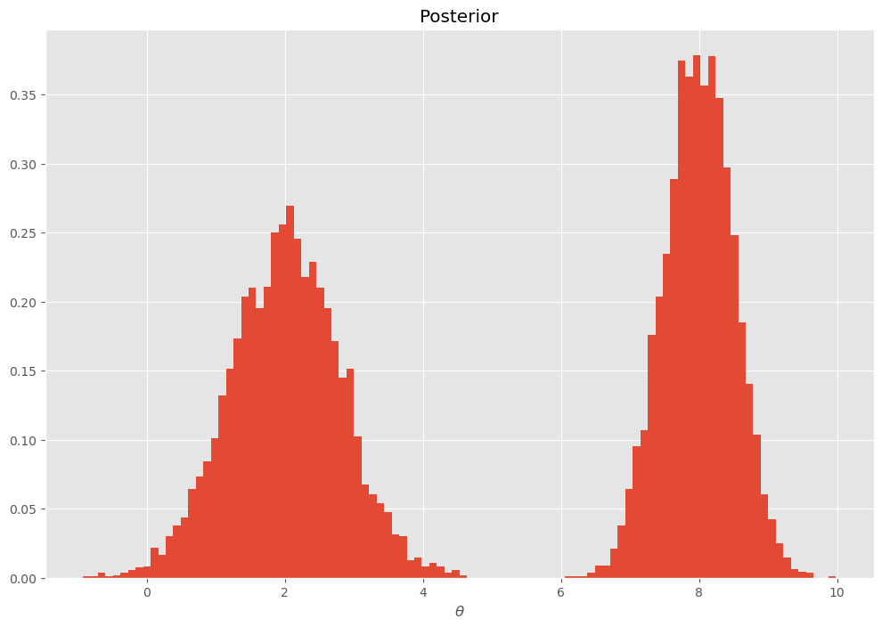
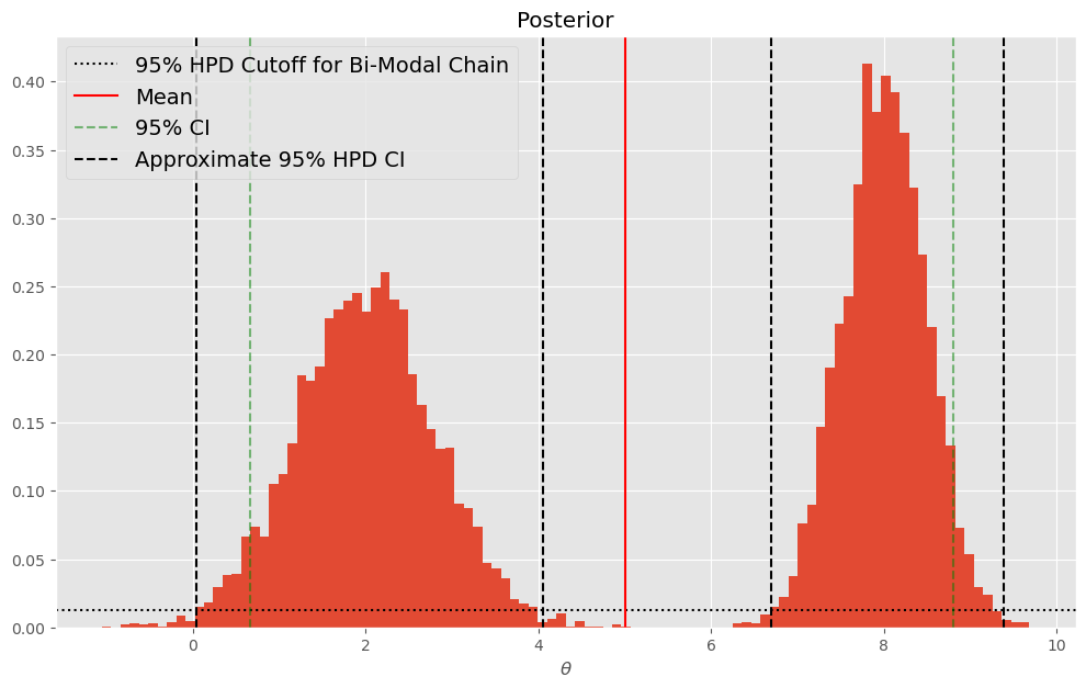
Applying the same principle, we can slide the horizontal dotted line down until we find the transition from low (\(<.025\)) and high regions of sampled parameters:

plt.figure(figsize=(12,7))
bimodal_chain = np.append(norm(2,.8).rvs(5000),norm(8,.5).rvs(5000))
plt.hist(bimodal_chain,bins=100, density=True)
plt.xlabel('$\\theta$')
plt.title('Posterior')
plt.axhline(.025/2,c='k',linestyle=':',label="95% HPD Cutoff for Bi-Modal Chain")
plt.axvline(bimodal_chain.mean(),c='r',label="Mean")
plt.axvline(np.percentile(bimodal_chain,2.5),c='g',linestyle='--',alpha=.5,label="95% CI")
plt.axvline(np.percentile(bimodal_chain,97.5),c='g',linestyle='--',alpha=.5)

plt.axvline(.05,c='k',linestyle='--',label="Approximate 95% HPD CI")
plt.axvline(4.05,c='k',linestyle='--')
plt.axvline(6.7,c='k',linestyle='--')
plt.axvline(9.39,c='k',linestyle='--')

plt.legend(loc='upper left', fontsize=14)
plt.show()

The Chain and MAP

How do the moments of our chain (e.g. mean and median) relate to MAP (parameter value that maximes the posterior)? To answer that question, we need to solve for MAP given the data:

def log_posterior(mu,data,sigma,mu_mu_prior,mu_sigma_prior):
    ln_prior = norm(mu_mu_prior,mu_sigma_prior).logpdf(mu)
    ln_like = norm(mu,sigma).logpdf(data).sum()
    return -1*(ln_like + ln_prior)

Using the negative log posterior, minimize to find MAP:

startvals = 9
from scipy.optimize import minimize
res = minimize(log_posterior,startvals, 
               args=(data,sigma,mu_prior,sigma_prior),options={'disp': True},
               method='BFGS')

Optimization terminated successfully.
         Current function value: 31.608815
         Iterations: 2
         Function evaluations: 6
         Gradient evaluations: 3

And here are the results:

print("The MAP is: ", res.x[0])
print("The mean of our sampled values is: ", chain[100:].mean())
print("The median is: ", np.percentile(chain[100:],50))

The MAP is:  10.160315804249501
The mean of our sampled values is:  10.180621628544616
The median is:  10.196002242838691

For well behaved symmetric posteriors, the mean of the posterior will usually be very close to MAP, but this doesn’t necessarily have to be the case. Note that in the preceding figure (the bimodal posterior), MAP is approximately 8 whereas the mean is approximately 5.