Maximum Likelihood Estimation in R
Contents
Maximum Likelihood Estimation in R#
This chapter shows how to setup a generic log-likelihood function in R and use that to estimate an econometric model. For ECON407, the models we will be investigating use maximum likelihood estimation and pre-existing log-likelihood definitions to estimate the model. Therefore, consider this chapter as NOT REQUIRED optional material.
The maximum likelihood method seeks to find model parameters \(\pmb{\theta}^{MLE}\) that maximizes the joint likelihood (the likelihood function- \(L\)) of observing \(\mathbf{y}\) conditional on some structural model that is a function of independent variables \(\mathbf{x}\) and model parameters \(\pmb{\theta}^{MLE}\):
In a simple ordinary least squares setting with a linear model, we have the model parameters \(\pmb{\theta}=[\pmb{\beta},\sigma]\) making the likelihood function
Typically, for computational purposes we work with the log-likelihood function rather than the the likelihood. This is
Load Data and run simple OLS regression Model#
# allows us to open stata datasets
library(foreign)
library(maxLik)
library(stargazer)
Loading our data:
tk.df = read.dta("http://rlhick.people.wm.edu/econ407/data/tobias_koop.dta")
tk4.df = subset(tk.df, time == 4)
tk4.df$ones=1
Linear Estimation of the OLS Model#
summary(lm(lm(ln_wage~educ + pexp + pexp2 + broken_home, data=tk4.df)))
Call:
lm(formula = lm(ln_wage ~ educ + pexp + pexp2 + broken_home,
    data = tk4.df))

Residuals:
     Min       1Q   Median       3Q      Max
-1.69490 -0.24818 -0.00079  0.25417  1.51139

Coefficients:
             Estimate Std. Error t value Pr(>|t|)
(Intercept)  0.460333   0.137294   3.353 0.000829 ***
educ         0.085273   0.009290   9.179  < 2e-16 ***
pexp         0.203521   0.023586   8.629  < 2e-16 ***
pexp2       -0.012413   0.002283  -5.438 6.73e-08 ***
broken_home -0.008725   0.035711  -0.244 0.807020
---
Signif. codes:  0 ‘***’ 0.001 ‘**’ 0.01 ‘*’ 0.05 ‘.’ 0.1 ‘ ’ 1

Residual standard error: 0.4265 on 1029 degrees of freedom
Multiple R-squared:  0.1664,	Adjusted R-squared:  0.1632
F-statistic: 51.36 on 4 and 1029 DF,  p-value: < 2.2e-16
Implementing Maximum Likelihood Estimation in R#
Here we define the likelihood function for an OLS model. Note the first step is to determine if the during optimization the numerical solver could allow the model variance \(\sigma^2<0\). If so, the model returns an NA (not a number), and the optimization function enters another iteration for looking for model parameters.
y = tk4.df$ln_wage
X = data.matrix(tk4.df[,c('educ', 'pexp', 'pexp2', 'broken_home', 'ones')],
                rownames.force = NA)
ols.lnlike <- function(theta) {
  if (theta[1] <= 0) return(NA)
  -sum(dnorm(y, mean = X %*% theta[-1], sd = sqrt(theta[1]), log = TRUE))
}
Note, that we can evaluate the log-likelihood for any parameter vector:
print(ols.lnlike(c(1,1,1,1,1,1)))
[1] 1305304
Manual Optimization (the hard way)#
While this method is the hard way, it demonstrates the mechanics of optimization in R. In order to find the best or optimal parameters, we use R’s optim function to find the estimated parameter vector. It needs as arguments
starting values
optimization method (for unconstrained problems
BFGSis a good choice)function to be minimized
any data that the function needs for evaluation.
Also, we can ask optim to return the hessian, which we’ll use for calculating standard errors.
mle_res.optim = optim(c(1,.1,.1,.1,.1,.1), method="BFGS",fn=ols.lnlike,hessian=TRUE)
summary(mle_res.optim)
            Length Class  Mode
par          6     -none- numeric
value        1     -none- numeric
counts       2     -none- numeric
convergence  1     -none- numeric
message      0     -none- NULL
hessian     36     -none- numeric
Our model parameters are
b = round(mle_res.optim$par,5)
print(b)
[1] 0.18106 0.08527 0.20352 -0.01241 -0.00873 0.46033
and the standard errors are
se = round(sqrt(diag(solve(mle_res.optim$hessian))),5)
print(se)
[1] 0.00796 0.00927 0.02353 0.00228 0.03562 0.13696
Putting it together for comparison to stata:
labels = c('Sigma2','educ','pexp','pexp2','broken_home','Constant')
tabledat = data.frame(matrix(c(labels,b,se),nrow=length(b)))
names(tabledat) = c("Variable","Parameter","Standard Error")
stargazer(tabledat,summary=FALSE,title="Maximum Likelihood Results from R",
          type="text",rownames = FALSE)
Maximum Likelihood Results from R
====================================
Variable    Parameter Standard Error
------------------------------------
Sigma2       0.18106     0.00796
educ         0.08527     0.00927
pexp         0.20352     0.02353
pexp2       -0.01241     0.00228
broken_home -0.00873     0.03562
Constant     0.46033     0.13696
------------------------------------
Using maxLik (the easy way)#
Unlike optim above, the maxLik package needs the log-likelihood value not -1*log-likelihood. So let’s redefine the likelihood:
ols.lnlike <- function(theta) {
  if (theta[1] <= 0) return(NA)
  sum(dnorm(y, mean = X %*% theta[-1], sd = sqrt(theta[1]), log = TRUE))
}
Using the maxLik package facilitates this process alot.
# starting values with names (a named vector)
start = c(1,.1,.1,.1,.1,.1)
names(start) = c("sigma2","educ","pexp","pexp2","broken_home","Constant")
mle_res <- maxLik( logLik = ols.lnlike, start = start, method="BFGS" )
summary(mle_res)
--------------------------------------------
Maximum Likelihood estimation
BFGS maximization, 114 iterations
Return code 0: successful convergence
Log-Likelihood: -583.6629
6  free parameters
Estimates:
             Estimate Std. error t value  Pr(> t)
sigma2       0.181058   0.007963  22.737  < 2e-16 ***
educ         0.085273   0.009262   9.207  < 2e-16 ***
pexp         0.203521   0.023527   8.651  < 2e-16 ***
pexp2       -0.012413   0.002277  -5.451    5e-08 ***
broken_home -0.008725   0.035626  -0.245 0.806525
Constant     0.460333   0.136879   3.363 0.000771 ***
---
Signif. codes:  0 ‘***’ 0.001 ‘**’ 0.01 ‘*’ 0.05 ‘.’ 0.1 ‘ ’ 1
--------------------------------------------
My personal opinion is that if you do a lot of this type of work (writing custom log-likelihoods), you are better off using Matlab, R, or Python than Stata. If you use R my strong preference is to use maxLik as I demonstrate above over mle or mle2, since the latter two require that you define your likelihood function as having separate arguments for each parameter to be optimized over.
Visualizing the Likelihood Function#
Let’s graph likelihood for the educ coefficient, holding
all data at observed values
other parameters constant at optimal values
I am going to call this a “marginal log-likelihood” since we are only allowing one parameter to vary in this plot (rather than all 6). Here is what it looks like:
coeff2 = mle_res.optim$par
altcoeff = seq(.06,.11,0.001)
LL = NULL

# calculates the LL for various values of the education parameter
# and stores them in LL:
for (m in altcoeff) {
  coeff2[2] = m # consider a candidate parameter value for education
  LLt = ols.lnlike(coeff2)
  LL = rbind(LL,LLt)
}


plot(altcoeff,LL, type="l", xlab="Education Coefficient", ylab="LogL",
     main="Marginal Log-Likelihood Function for \n Education Coefficient")

abline(v=mle_res$estimate[2], col="red")
abline(h=mle_res$maximum, col="red")
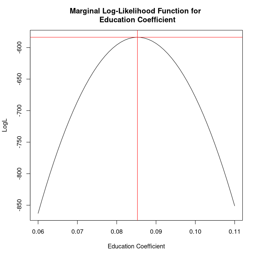
This shows that the parameter value of .085 maximizes the log-likelihood function.