OLS in R
Contents
OLS in R#
This document shows how to implement the topics we cover in cross-section econometrics in R.
# allows us to open stata datasets
library(foreign)
# for heteroskedasticity corrected variance/covariance matrices
library(sandwich)
# for White Heteroskedasticity Test
library(lmtest)
# for very pretty tables
library(stargazer)
# for bootstrapping
library(boot)
Load data and summarize:
tk.df = read.dta("http://rlhick.people.wm.edu/econ407/data/tobias_koop.dta")
tk4.df = subset(tk.df, time == 4)
stargazer(tk4.df,header=FALSE,title="Tobias and Koop Summary Statistics", type='text')
Tobias and Koop Summary Statistics
=================================================
Statistic     N     Mean    St. Dev.  Min    Max
-------------------------------------------------
id          1,034 1,090.952 634.892    4    2,177
educ        1,034  12.275    1.567     9     19
ln_wage     1,034   2.138    0.466   0.420  3.590
pexp        1,034   4.815    2.190     0     12
time        1,034   4.000    0.000     4      4
ability     1,034   0.017    0.921   -3.140 1.890
meduc       1,034  11.403    3.027     0     20
feduc       1,034  11.585    3.736     0     20
broken_home 1,034   0.169    0.375     0      1
siblings    1,034   3.200    2.127     0     15
pexp2       1,034  27.980    22.599    0     144
-------------------------------------------------
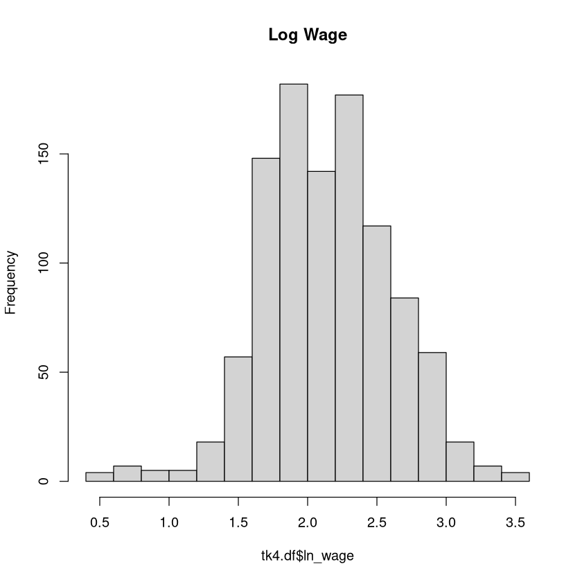
Focusing on our dependent variable:
hist(tk4.df$ln_wage,main = "Log Wage")
The OLS Model#
In R we use
ols.lm = lm(ln_wage~educ + pexp + pexp2 + broken_home, data=tk4.df)
summary(ols.lm)
Call:
lm(formula = ln_wage ~ educ + pexp + pexp2 + broken_home, data = tk4.df)

Residuals:
     Min       1Q   Median       3Q      Max
-1.69490 -0.24818 -0.00079  0.25417  1.51139

Coefficients:
             Estimate Std. Error t value Pr(>|t|)
(Intercept)  0.460333   0.137294   3.353 0.000829 ***
educ         0.085273   0.009290   9.179  < 2e-16 ***
pexp         0.203521   0.023586   8.629  < 2e-16 ***
pexp2       -0.012413   0.002283  -5.438 6.73e-08 ***
broken_home -0.008725   0.035711  -0.244 0.807020
---
Signif. codes:  0 ‘***’ 0.001 ‘**’ 0.01 ‘*’ 0.05 ‘.’ 0.1 ‘ ’ 1

Residual standard error: 0.4265 on 1029 degrees of freedom
Multiple R-squared:  0.1664,	Adjusted R-squared:  0.1632
F-statistic: 51.36 on 4 and 1029 DF,  p-value: < 2.2e-16
Robust Standard Errors#
Note that since the \(\mathbf{b}\)’s are unbiased estimators for \(\beta\), those continue to be the ones to report. However, our variance covariance matrix is $\( VARCOV_{HC1} = \mathbf{(x'x)^{-1}\hat{V}(x'x)^{-1}} \)$
Defining \(\mathbf{e=y-xb}\), $\( \hat{\mathbf{V}} = diag(\mathbf{ee}') \)$
Implementing this in R, we can use the sandwich package’s vcovHC function with the HC1 option (stata default):
VARCOV = vcovHC(ols.lm, 'HC1')
se = sqrt(diag(VARCOV))
print(se)
(Intercept)        educ        pexp       pexp2 broken_home
0.131541623 0.009929445 0.022683530 0.002244678 0.031238081
Note that the F-statistic reported by OLS is inappropriate in the presence of heteroskedasticity. We need to use a different form of the F test. Stata does this automatically. In R, we need to use waldtest for the correct model F statistic:
waldtest(ols.lm, vcov = vcovHC(ols.lm,'HC1'))
| Res.Df | Df | F | Pr(>F) | |
|---|---|---|---|---|
| <dbl> | <dbl> | <dbl> | <dbl> | |
| 1 | 1029 | NA | NA | NA |
| 2 | 1033 | -4 | 64.81968 | 6.411661e-49 |
We can put this together to make a more useful summary output:
# copy summary object
robust.summ = summary(ols.lm)
# overwrite all coefficients with robust counterparts
robust.summ$coefficients = unclass(coeftest(ols.lm, vcov. = VARCOV))
# overwrite f stat with correct robust value
f_robust = waldtest(ols.lm, vcov = VARCOV)
robust.summ$fstatistic[1] = f_robust$F[2]
print(robust.summ)
Call:
lm(formula = ln_wage ~ educ + pexp + pexp2 + broken_home, data = tk4.df)

Residuals:
     Min       1Q   Median       3Q      Max
-1.69490 -0.24818 -0.00079  0.25417  1.51139

Coefficients:
             Estimate Std. Error t value Pr(>|t|)
(Intercept)  0.460333   0.131542   3.500 0.000486 ***
educ         0.085273   0.009929   8.588  < 2e-16 ***
pexp         0.203521   0.022684   8.972  < 2e-16 ***
pexp2       -0.012413   0.002245  -5.530 4.06e-08 ***
broken_home -0.008725   0.031238  -0.279 0.780057
---
Signif. codes:  0 ‘***’ 0.001 ‘**’ 0.01 ‘*’ 0.05 ‘.’ 0.1 ‘ ’ 1

Residual standard error: 0.4265 on 1029 degrees of freedom
Multiple R-squared:  0.1664,	Adjusted R-squared:  0.1632
F-statistic: 64.82 on 4 and 1029 DF,  p-value: < 2.2e-16
The Bootstrapping Approach#
In what follows below, I should you how to use R for bootstrapping regression coefficients, which will fix any heteroskedasticity problems we might have.
bs_ols <- function(formula, data, indices) {
  d <- data[indices,] # allows boot to select sample
  fit <- lm(formula, data=d)
  return(coef(fit))
}

results <- boot(data=tk4.df, statistic=bs_ols,
  	R=1000, formula=ln_wage~educ + pexp + pexp2 + broken_home)

boot.ci(results,conf=0.95,type='perc',index=1)
boot.ci(results,conf=0.95,type='perc',index=2)
boot.ci(results,conf=0.95,type='perc',index=3)
boot.ci(results,conf=0.95,type='perc',index=4)
boot.ci(results,conf=0.95,type='perc',index=5)

colnames(results$t) = c("Intercept","educ","pexp","pexp2","broken_home")
summary(results$t)
BOOTSTRAP CONFIDENCE INTERVAL CALCULATIONS
Based on 1000 bootstrap replicates

CALL :
boot.ci(boot.out = results, conf = 0.95, type = "perc", index = 1)

Intervals :
Level     Percentile
95%   ( 0.2106,  0.7247 )
Calculations and Intervals on Original Scale
BOOTSTRAP CONFIDENCE INTERVAL CALCULATIONS
Based on 1000 bootstrap replicates

CALL :
boot.ci(boot.out = results, conf = 0.95, type = "perc", index = 2)

Intervals :
Level     Percentile
95%   ( 0.0645,  0.1035 )
Calculations and Intervals on Original Scale
BOOTSTRAP CONFIDENCE INTERVAL CALCULATIONS
Based on 1000 bootstrap replicates

CALL :
boot.ci(boot.out = results, conf = 0.95, type = "perc", index = 3)

Intervals :
Level     Percentile
95%   ( 0.1593,  0.2475 )
Calculations and Intervals on Original Scale
BOOTSTRAP CONFIDENCE INTERVAL CALCULATIONS
Based on 1000 bootstrap replicates

CALL :
boot.ci(boot.out = results, conf = 0.95, type = "perc", index = 4)

Intervals :
Level     Percentile
95%   (-0.0168, -0.0080 )
Calculations and Intervals on Original Scale
BOOTSTRAP CONFIDENCE INTERVAL CALCULATIONS
Based on 1000 bootstrap replicates

CALL :
boot.ci(boot.out = results, conf = 0.95, type = "perc", index = 5)

Intervals :
Level     Percentile
95%   (-0.0695,  0.0489 )
Calculations and Intervals on Original Scale
   Intercept            educ              pexp            pexp2
 Min.   :0.04771   Min.   :0.05564   Min.   :0.1316   Min.   :-0.01988
 1st Qu.:0.37305   1st Qu.:0.07856   1st Qu.:0.1877   1st Qu.:-0.01401
 Median :0.46360   Median :0.08527   Median :0.2035   Median :-0.01236
 Mean   :0.46230   Mean   :0.08513   Mean   :0.2035   Mean   :-0.01241
 3rd Qu.:0.55261   3rd Qu.:0.09202   3rd Qu.:0.2196   3rd Qu.:-0.01081
 Max.   :0.84488   Max.   :0.12228   Max.   :0.2846   Max.   :-0.00548
  broken_home
 Min.   :-0.107363
 1st Qu.:-0.029781
 Median :-0.009216
 Mean   :-0.009060
 3rd Qu.: 0.011689
 Max.   : 0.083809
Testing for Heteroskedasticity#
The two dominant heteroskedasticity tests are the White test and the Cook-Weisberg (both Breusch Pagan tests). The White test is particularly useful if you believe the error variances have a potentially non-linear relationship with model covariates.
In R we perform the White test by:
bptest(ols.lm,ln_wage ~ educ*pexp + educ*pexp2 + educ*broken_home +
                        pexp*pexp2 + pexp*broken_home + pexp2*broken_home +
                        I(educ^2) + I(pexp^2) + I(pexp2^2) + I(broken_home^2),
       data=tk4.df)
	studentized Breusch-Pagan test

data:  ols.lm
BP = 29.196, df = 12, p-value = 0.003685
Notice that in R, we need to specify the form of the heteroskedasticity. To mirror the White test, we include interaction and second order terms. Both stata’s imtest and R’s bptest allow you to specify more esoteric forms of heteroskedasticity, although in R it is more apparent since we have to specify the form of the heteroskedasticity for the test to run.
A more basic test- one assuming that heteroskedastity is a linear function of the \(\mathbf{x}\)’s- is the Cook-Weisberg Breusch Pagan test. R doesn’t implement this test directly. But it can be performed manually following the steps we discussed in class:
Recover residuals as above, denote as \(\mathbf{e}\)
square the residuals by the sqare root of mean squared residuals: $\( \mathbf{r} = \frac{diagonal(\mathbf{ee}')}{\sqrt{\mathbf{e'e}/N}} \)$
Run the regression \(\mathbf{r} = \gamma_0 + \gamma_1 \mathbf{xb} + \mathbf{v}\). Recall that \(\mathbf{xb} = \mathbf{\hat{y}}\).
Recover ESS defined as $\( ESS = (\mathbf{\hat{r}} - \bar{r})'(\hat{\mathbf{r}} - \bar{r}) \)$
ESS/2 is the test statistic distributed \(\chi^2_{(1)}\)