import numpy as np
from scipy.stats import norm,uniform
import matplotlib.pyplot as plt
import seaborn as sbn
import pandas as pd

np.random.seed(282629734)

plt.style.use('ggplot')

Convergence Diagnostics and Model Checks

From the previous notebook, we know that using MH leads to a Markov Chain that we can use for inference. This is predicated on our chain converging to our stationary distribution (the posterior). Knowing when a chain has converged is a numerical issue and there are some important diagnostic tools we’ll be using for assessing convergence.

Note

For empirical Bayesian analysis, the two biggest challenges are ensuring that

1. Ergodicity is met

2. Your chain (sample parameter values) has converged

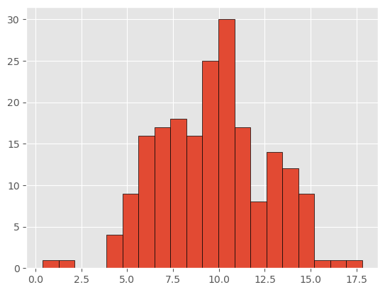
For having some data to play with, let’s resurrect our simple example yet again:

sigma = 3          # Note this is the *known* std of x
y = norm(10,sigma).rvs(200)
mu_prior = 8
sigma_prior = 1.5  # Note this is our prior on the std of mu

plt.hist(y, bins=20, edgecolor='k')
plt.show()

For sampling purposes, let’s recycle our simple 1-parameter sampler:

# a fairly basic mh mcmc random walk sampler:
def sampler(data, samples=4, mu_init=9, sigma= 1, proposal_width=3, 
            mu_prior_mu=10, mu_prior_sd=1):
    mu_current = mu_init
    posterior = [mu_current]
    
    posterior = np.zeros(samples)
    
    for i in range(samples):
        # suggest new position
        mu_proposal = norm(mu_current, proposal_width).rvs()

        # Compute likelihood by multiplying probabilities of each data point
        likelihood_current = norm(mu_current, sigma).pdf(data).prod()
        likelihood_proposal = norm(mu_proposal, sigma).pdf(data).prod()
        
        # Compute prior probability of current and proposed mu        
        prior_current = norm(mu_prior_mu, mu_prior_sd).pdf(mu_current)
        prior_proposal = norm(mu_prior_mu, mu_prior_sd).pdf(mu_proposal)
        
        p_current = likelihood_current * prior_current
        p_proposal = likelihood_proposal * prior_proposal
        
        # Accept proposal?
        c = np.min((1,p_proposal / p_current))
        
        accept = np.random.rand() <= c
                
        if accept:
            # Update position
            mu_current = mu_proposal
        
        posterior[i] = mu_current
        
    return np.array(posterior)

And let’s sample 5000 times from the posterior:

chain = sampler(y, samples=5000, mu_init=9, sigma=sigma, proposal_width=2,
                mu_prior_mu=mu_prior, mu_prior_sd=sigma_prior)

Let’s examine the trace and histogram of the chain:

plt.figure(figsize=(15,6))
plt.subplot(121)
plt.plot(np.arange(chain.shape[0]),chain)
plt.axhline(np.mean(chain),linestyle='--',c='k')
plt.title('Trace Plot for $\\mu$')

plt.subplot(122)
plt.hist(chain,orientation='horizontal',bins=30, edgecolor='k')
plt.axhline(np.mean(chain),linestyle='--', c='k')
plt.title('Histogram for $\\mu$')

plt.tight_layout()
plt.show()

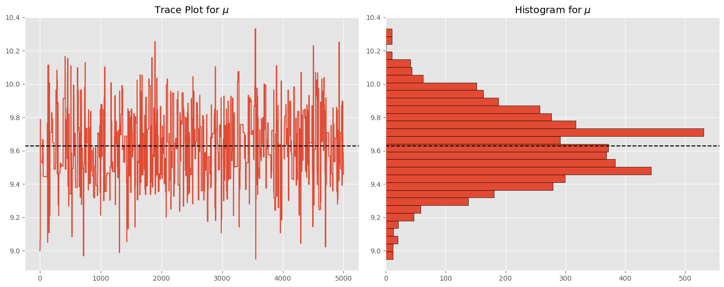
How do we know this chain has converged to the posterior?

This is the fundamental question we are addressing in this chapter. Below we present several approaches and in practice you would want to explore each of these since convincing your audience of chain convergence is so fundamental to work in empirical Bayesian analysis. These approaches are

1. Visual Inspection of trace

2. Simulation Error

3. Examining autocorrelation plots

4. Ensuring your chain has appropriate acceptance rates

5. Convergence diagnostics:

   • Gelman-Rubin

   • Geweke

   • Raftery-Lewis

Sampling Error

This investigates the question how does the mean of \(\theta\) deviates in our chain, and is capturing the simulation error of the mean rather than underlying uncertainty of our parameter \(\theta\):

\[ SE^{\bar{\theta}} = \frac{\sum_{i=1}^B \sqrt{\sum_{j =1}^{J_i}\frac{(\mu_j - \bar{\mu}_i)^2}{J_i}}}{\sqrt{B}} \]

where \(B\) is the number of batches and \(J_i\) is the number of samples in batch \(i\). Note that the package we’ll be using calls this ``MC Error’’.

Defining the function for calculating simulation error as:

# this is a trimmed version of mc_error from
#    arviz, for a single parameter
def mc_error(chain, batches):
    batched_traces = np.resize(chain, (batches, int(len(chain) / batches)))
    means = np.mean(batched_traces, 1)
    std = np.std(means)
    return std / np.sqrt(batches)

For our problem, this is:

print("MC Error: ", mc_error(chain, 10).round(5)) 
print("Std error of Samples: ", np.std(chain).round(5))

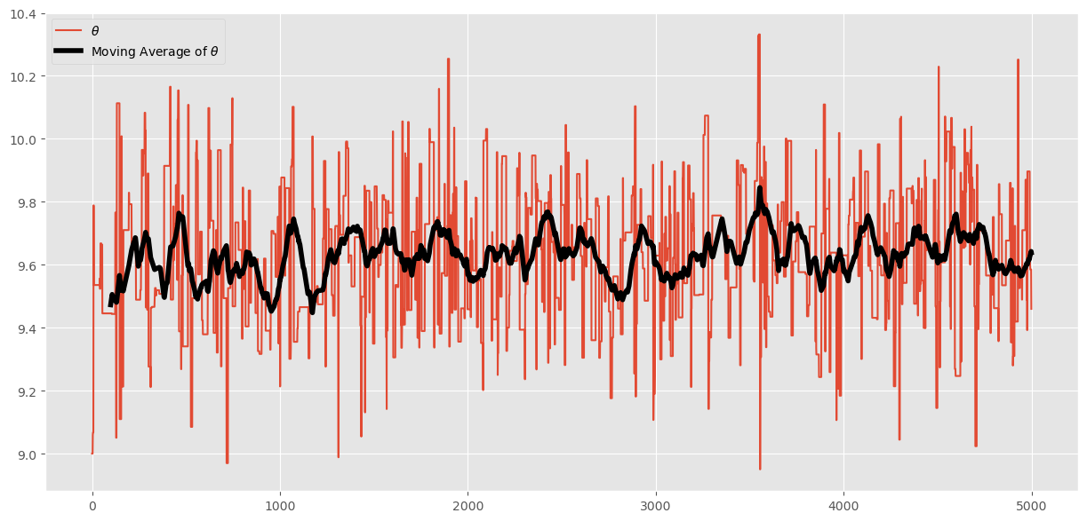
MC Error:  0.00864
Std error of Samples:  0.21536

This is saying that very little of our posterior variation in \(\theta\) is due to sampling error (that is good). We can visualize this by examining the moving average of our chain as we move through the 5000 iterations:

# pandas makes this easy:
df_chain = pd.DataFrame(chain,columns=['theta'])
df_chain['ma_theta'] = df_chain['theta'].rolling(100).mean()
ax = df_chain.plot(figsize=(15,7))
ax.lines[-1].set_linewidth(4)
ax.lines[-1].set_color('k')
ax.lines[0].set_label("$\\theta$")
ax.lines[-1].set_label("Moving Average of $\\theta$")
plt.legend()
plt.show()

Autocorrelation, Effective Sample Size, and Thinning

An extremely important consideration is to what degree our samples are correlated across draws. We can judge this visually (plotting autocorrelation) and calculating the ESS, the effective sample size.

Thinning is also a method- no longer commonly used- for reducing autocorrelation in monte carlo markov chains.

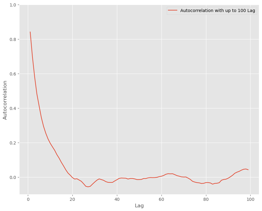
Autocorrelation Plots

We examined these briefly in the previous chapter. For slow mixing chains, autocorrelation plots could indicate that your chain has failed to reach regions of the parameter space near the bulk of the probability mass in your posterior or that it is inefficiently exploring the chain.

We will again use the custom autocorrelation function from before:

# an autocorrelation function for a given length
# returns autocorrelation of period t with t, t-1, t-2, ..., t-L 
# from https://stackoverflow.com/questions/643699/how-can-i-use-numpy-correlate-to-do-autocorrelation
def acf(x, length=20):
    return np.array([1]+[np.corrcoef(x[:-i], x[i:])[0,1]  \
        for i in range(1, length)])

lags=np.arange(1,100)

fig, ax = plt.subplots(figsize=(10,8))
ax.plot(lags, acf(chain, 100)[1:], label='Autocorrelation with up to 100 Lag')
ax.legend(loc=0)
_ = ax.set(xlabel='Lag', ylabel='Autocorrelation', ylim=(-.1, 1))
sbn.despine()
plt.show()

Effective sample size

The effective sample size is the number of samples, if drawn form iid variates, necessary to achieve the same amount of information about the posterior when drawn from correlated samples from the posterior. Usually (but not always) the effective sample size is less than the amount of samples in your chain.

The effective sample size (\(N_{eff}\)) given by the equation

\[ N_{eff} = \frac{N}{1 + 2\sum_{t=1}^\infty\rho_t} \]

where \(\rho_t\) is the autocorrelation between the current time period and \(t\) periods forward.

In practice our chain does not contain infinite number of samples. So it is approximated using a finite measure of the above, similar to the calculations below:

rho = acf(chain, 100)[1:]
N = chain.shape[0]

print("Sample size: ", N)
print("Effective sample size: ", N / (1 + 2 * rho.sum())) 

Sample size:  5000
Effective sample size:  522.0453411450135

Thinning

Thinning samples is a practice of keeping every \(k^th\) sample. For example if the following are samples from your posterior:

\[ {1, 2, 3, 4, 5, 6, 7, 8, 9, 10, 11, 12, 13} \]

and the chain is thinned by retaining every \(3^{rd}\) sample, the thinned sample would be

\[ {1, 4, 7, 10, 13} \]

Historically this practice was used to

1. Reduce autocorrelation when using Metropolis-Hastings random walk step methods

2. Reduce computer memory/disk space requirements of storing every sample

More modern step methods have made the practice of thinning something rarely done on modern computer hardware.

Acceptance Rate of the Metropolis-Hasting algorithm

Recall that we want the acceptance rate to be in the range .2 to .5. For our problem this paper suggests an acceptance rate of .234 for random walk MH.

Since the number of new members in the chain represent the number of acceptances, count changes in chain values and divide by total chain length to calculate acceptance rate:

changes = np.sum((chain[1:]!=chain[:-1]))
print("Acceptance Rate is: ", changes/(chain.shape[0]-1))

Acceptance Rate is:  0.1300260052010402

The acceptance rate is helpful in describing convergence because it indicates a good level of “mixing” over the parameter space. Here the acceptance rate is too low, so we should decrease proposal width and re-run our MH MCMC sampler.

Note: modern software (like PyMC) can auto-tune \(\omega\) to achieve a desired acceptance rate. We don’t have that capability in the sampler we have defined above.

Convergence Diagnostics

These (particularly Gelman-Rubin and Geweke) are the ones to rely on most for determining chain convergence.

Gelman-Rubin Diagnostic

If our MH MCMC Chain reaches a stationary distribution, and we repeat the excercise multiple times, then we can examine if the posterior for each chain converges to the same place in the distribution of the parameter space.

Steps:

1. Run \(M>1\) Chains of length \(2 \times N\).

2. Discard the first \(N\) draws of each chain, leaving \(N\) iterations in the chain (The first \(N\) observations are often called “burn-in” observations).

3. Calculate the within and between chain variance.

   • Within chain variance:

     \[ W = \frac{1}{M}\sum_{j=1}^M s_j^2 \]

     where \(s_j^2\) is the variance of each chain (after throwing out the first \(N\) draws).

   • Between chain variance:

     \[ B = \frac{N}{M-1} \sum_{j=1}^M (\bar{\theta_j} - \bar{\bar{\theta}})^2 \]

     where \(\bar{\bar{\theta}}\) is the mean of the parameter across all \(M\) chains.

4. Calculate the estimated variance of \(\theta\) as the weighted sum of between and within chain variance.

   \[ \hat{var}(\theta) = \left ( 1 - \frac{1}{N}\right ) W + \frac{1}{N}B \]

5. Calculate the potential scale reduction factor.

   \[ \hat{R} = \sqrt{\frac{\hat{var}(\theta)}{W}} \]

We want this number to be close to 1. Why? This would indicate that the between chain variance is small. This makes sense, if between chain variance is small, that means both chains are mixing around the stationary distribution. Gelmen and Rubin show that when \(\hat{R}\) is greater than 1.1 or 1.2, we need longer burn-in.

This diagnostic requires multiple sampling runs, the more the better. Here we compute this over 2 chains. In your own work, you would probably want more than 2 (the default in PyMC is equal to the number of processor cores available). Sampling 5000 samples twice:

chain1 = sampler(y, samples=5000, mu_init=9, sigma=sigma, proposal_width=2,
                mu_prior_mu=mu_prior,mu_prior_sd = sigma_prior)
chain2 = sampler(y, samples=5000, mu_init=9, sigma=sigma, proposal_width=2,
                mu_prior_mu=mu_prior,mu_prior_sd = sigma_prior)

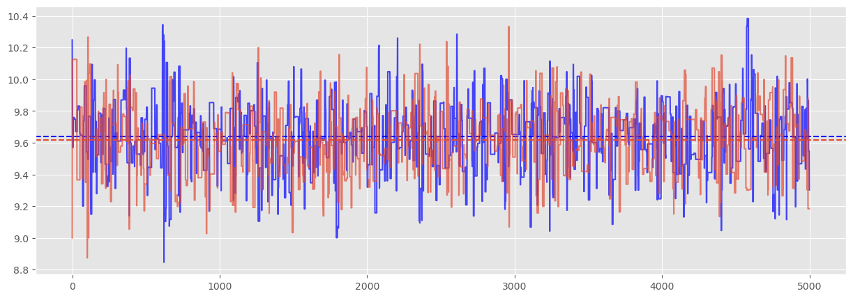
Visually, we can inspect the trace and see that we would expect the diagnostic to confirm chain convergence:

plt.figure(figsize=(15,5))
plt.plot(np.arange(5000),chain1, c='blue', alpha=.7)
plt.axhline(chain1.mean(), ls='--', c='blue')
plt.plot(np.arange(5000),chain2,alpha=.7)
plt.axhline(chain2.mean(), ls='--');

The Gelman-Rubin diagnostic is

# here we toss the first half of our samples for "burnin
N = int(chain.shape[0]/2)

W = (chain1[-N:].std()**2 + chain2[-N:].std()**2)/2
mean1 = chain1[-N:].mean()
mean2 = chain2[-N:].mean()
mean = (mean1 + mean2)/2
B = N * ((mean1 - mean)**2 + (mean2 - mean)**2)
var_theta = (1 - 1/N) * W + 1/N*B
print("Gelmen-Rubin Diagnostic: ", np.sqrt(var_theta/W))

Gelmen-Rubin Diagnostic:  1.0009271513032512

Which confirms convergence. When we begin using the PyMC package, we won’t need to manually code this in python.

It should be evident that Gelmen-Rubin has two factors at play: burn-in and chain length. Really this criteria can be used ex-post to justify decisions on burn-in and chain length.

Geweke Diagnostic

We can explicitly think of this test as a test for the Ergodicity (stationarity) of your chain. This test only requires one chain rather than multiples as in Gelman-Rubin.

Take the first 10 and last 50% of your chain and do a t test comparing means (correcting for autocorrelation). Software packages, take this a step further: The geweke function in pymc2 by default chooses the first 10% of your chain, and the final 50%; divides the final 50% of the chain into 20 segments and performs a z-test for each segment. You want to fail to reject the null, since the hypothesis is:

\[\begin{split} H_0: \theta_{10\%} = $\theta^s_{50\%} \\ H_1: \theta_{10\%} \ne $\theta^s_{50\%} \end{split}\]

for each segment \(s\). If our means are the same (we fail to reject the null), then we have strong evidence of chain convergence.

This function has recently been removed from PyMC since the preferred method is Gelman-Rubin (previous section). However, to me this diagnostic test has a lot of value in thinking about ergodicity. Here is a “custom” function for the Geweke diagnostic:

def geweke(x, first=.1, last=.5, intervals=20, maxlag=20):
    """Return z-scores for convergence diagnostics.
    Compare the mean of the first % of series with the mean of the last % of
    series. x is divided into a number of segments for which this difference is
    computed. If the series is converged, this score should oscillate between
    -1 and 1.
    
    Taken from https://github.com/pymc-devs/pymc2/blob/master/pymc/diagnostics.py
    
    Parameters
    ----------
    x : array-like
      The trace of some stochastic parameter.
    first : float
      The fraction of series at the beginning of the trace.
    last : float
      The fraction of series at the end to be compared with the section
      at the beginning.
    intervals : int
      The number of segments.
    maxlag : int
      Maximum autocorrelation lag for estimation of spectral variance
    Returns
    -------
    scores : list [[]]
      Return a list of [i, score], where i is the starting index for each
      interval and score the Geweke score on the interval.
    Notes
    -----
    The Geweke score on some series x is computed by:
      .. math:: \frac{E[x_s] - E[x_e]}{\sqrt{V[x_s] + V[x_e]}}
    where :math:`E` stands for the mean, :math:`V` the variance,
    :math:`x_s` a section at the start of the series and
    :math:`x_e` a section at the end of the series.
    References
    ----------
    Geweke (1992)
    """
    from statsmodels.regression.linear_model import yule_walker
    
    def spec(x, order=2):
        beta, sigma = yule_walker(x, order)
        return sigma**2 / (1. - np.sum(beta))**2
    
    if np.ndim(x) > 1:
        return [geweke(y, first, last, intervals) for y in np.transpose(x)]

    # Filter out invalid intervals
    if first + last >= 1:
        raise ValueError(
            "Invalid intervals for Geweke convergence analysis",
            (first, last))

    # Initialize list of z-scores
    zscores = [None] * intervals

    # Starting points for calculations
    starts = np.linspace(0, int(len(x)*(1.-last)), intervals).astype(int)

    # Loop over start indices
    for i,s in enumerate(starts):

        # Size of remaining array
        x_trunc = x[s:]
        n = len(x_trunc)

        # Calculate slices
        first_slice = x_trunc[:int(first * n)]
        last_slice = x_trunc[int(last * n):]

        z = (first_slice.mean() - last_slice.mean())
        z /= np.sqrt(spec(first_slice)/len(first_slice) +
                     spec(last_slice)/len(last_slice))
        zscores[i] = len(x) - n, z
        
    # convert odd tuple setup to ndarray
    zscores_ = [[zi[0], zi[1]] for zi in zscores]
    return np.array(zscores_)

And we can plot the z scores to examine if the means for various segments are different from the first 50% of our chain:

plt.figure(figsize=(10,6))
gw_plot = geweke(chain)
plt.scatter(gw_plot[:,0],gw_plot[:,1])
plt.axhline(-1.98, c='r')
plt.axhline(1.98, c='r')
plt.ylim(-3.5,3.5)
plt.title('Geweke Plot Comparing first 10% and Slices of the Last 50% of Chain')
plt.xlim(-10,2510)
plt.show()

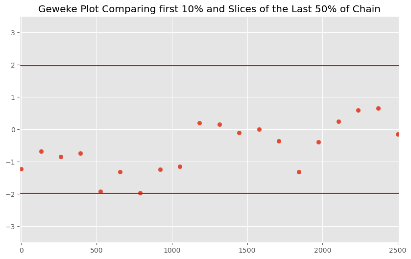
Even without dropping any burn-in observations (e.g. excluding the first 1000 samples), we have convergence. We only start seeing issues when we restrict ourselves to the first 5 values in the chain. Suggests we should drop the first few dozen observations for burn-in.

Apart from this being a univariate diagnostic (as all of these are), the primary criticism is that this test is viewed as inferior to Gelman-Rubin, since we could have found z-scores associated with ergodicity by chance for this single chain. Furthermore, since often time costs of additional chains are often negligible common practice is to focus solely on Gelman-Rubin.

Raftery-Lewis

This diagnostic is no longer used very much and I won’t cover it here.

Univariate Approaches

The diagnosticss we have discussed are all univariate (they work perfectly when there is only 1 parameter to estimate). Other diagnostics have been derived for the multivariate case, but these are useful only when using Gibbs Samplers or other specialized versions of Metropolis-Hastings.

So most people examine univariate diagnostics for each variable, examine autocorrelation plots, acceptance rates and try to argue chain convergence based on that- unless they are using Gibbs or other specialized samplers and can apply the more specialized multivariate tests.

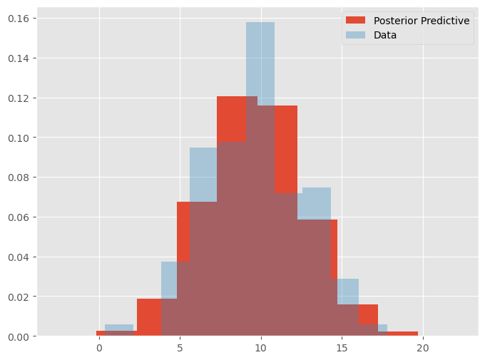
Posterior Predictive Checks

Another useful check is to see if the samples from your posterior can generate data (independent variable) that looks like the data used for estimation.

This check is not useful for assessing convergence but can identify how well your posterior exploration is unfolding and examines the predictive capability of your model.

This is probably a more useful concept for multivariate models, than the simple model for the mean we are exploring here. Still it is useful to apply the concept manually to see how it works (since later we will use automatically generated posterior predictives.

# note, the chain has multiple samples for the mean. For each 
# sample, generate yhat for each observation

# to make this manageable only use last 100 draws
check_mu = chain[-100:]

# generate synthetic data, conditional
# on each sample
pp_mu = norm(check_mu, sigma * np.ones(check_mu.shape[0])).rvs((y.shape[0], check_mu.shape[0]))
print("Note the shape has rows equal to the number of data "+
      "values and columns equal to number of samples: ", pp_mu.shape)

Note the shape has rows equal to the number of data values and columns equal to number of samples:  (200, 100)

plt.figure(figsize=(8, 6))
plt.hist(pp_mu.flatten(), label = "Posterior Predictive", density=True)
plt.hist(y, label = "Data", density=True, alpha=.35)
plt.legend()
plt.show()

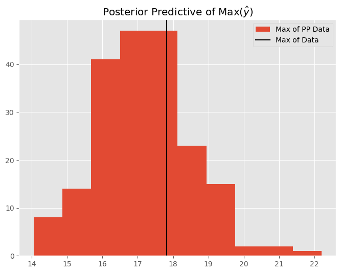
We can also perform checks over other statistics such as the maximum, minimum, or standard deviation of the data. We can use the posterior predictive distribution to show us how the model performs with the data it generates. Let’s examine the maximum predicted data value:

# calculate sigma (std of data) for each of the 100 samples
sigma_pp = pp_mu.max(axis=-1)
plt.figure(figsize=(8,6))
plt.title(r'Posterior Predictive of Max($\hat{y}$)')
plt.hist(sigma_pp, label='Max of PP Data')
plt.axvline(y.max(), label='Max of Data', c='k')
plt.legend()
plt.show()

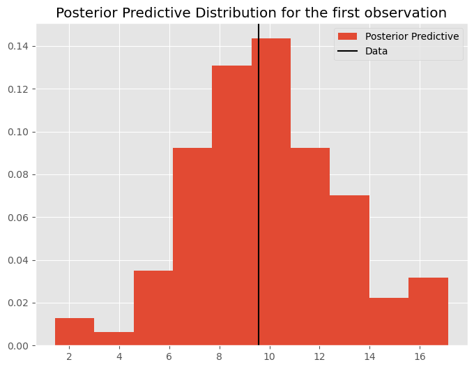
These examples are fairly trivial for the 1 parameter estimation problem we have here. However as we move to more interesting problems, posterior predictive checks are extremely good for examining not only predictive capabilities of your model, but diagnosing problematic observations or outliers where the model is struggling to fit the data. Note that the posterior predictive distribution of data is generated for every observation:

plt.figure(figsize=(8, 6))
plt.title('Posterior Predictive Distribution for the first observation')
plt.hist(pp_mu[:,0], label = "Posterior Predictive", density=True)
plt.axvline(y[0], label = "Data", c='k')
plt.legend()
plt.show()

Finally, we will see in later lectures that posterior predictives can help with diagnosing the degree to which your prior is “pulling” your posterior away from the likelihood.

Burn-in

Another extremely important concept is called burn-in. This refers to the amount of samples necessary for the sampler to reach regions of the parameter space relavant for proper sampling from your posterior, and these samples are discarded as they can be viewed as samples that can’t provide useful information about the posterior. Nearly every problem requires some amount of burn-in. Unfortunately, the quantity of burn-in observations is unknown a priori so often researchers will run chains for a long time (overnight) collecting all samples and then using the techniques above to define a burn-in breakpoint. Fortunately, modern samplers- better than the random-walk Metropolis Hastings one we have been using- require very little burn-in.