%matplotlib inline
import re as re
import pandas as pd
import numpy as np
import seaborn as sbn
from scipy.stats import norm
import matplotlib.pyplot as plt

sbn.set_style('white')
sbn.set_context('talk')

np.random.seed(12345678)
Introduction to PyMC#
Note
Note: the description of software in this introduction are my personal opinions and I’m sure that lots of people would disagree with my assessment of available software packages.
We have been working on getting under the hood of Metropolis-Hastings and Monte Carlo Markov Chain. But there are some very accessible Metropolis Markov Chain software packages out there. These are my personal views on what is available:
Stata (
bayesianmh)- just available in Stata 14. To be honest, I have never heard of anyone using Stata for Bayesian Sampling Methods although I haven’t really looked.Matlab. There are numerous user and Matlab written routines. For example, there is a version of
emceethat is implemented there (more on this later in the course). Matlab is for people who want to possibly tweak their own sampler code and who need the fastest possible computation.SAS. A decent set of packages, not used very much in the social sciences (maybe in the medical sciences??), but is well suited for big data.
R. For a long time R was the de-facto standard and probably still is, with packages like
R-stanwhich interfaces theSTANC Library. Another big advantage to usingR-stanis that Gelman is an active contributer to that package. AlsoJags,RbugsandOpen BUGShave been around for a long time. I almost elected to teach this course in R.Python. The libraries aren’t as rich as R, but you might view Python as sitting between Matlab and R. Maybe (in my view probably) faster and also easier to code your own samplers than R. Python is the de facto language for many applied physicists, and they need speed and the latest samplers. Additionally Python is strong in the big-data environment, more so than any of the other packages mentioned above. The major players on python are:
PyMC
PyStan
EMCEE
Tensorflow Probability
PyTorch
Jax (not exactly a Bayesian library, but often useful)
These final three packages are also optimized to use graphical processors (GPUs) which can result in massive speedups for computationally expensive models.
Today, we are going to focus on PyMC, which is a very easy to use package now that we have a solid understanding of how posteriors are constructed.
We will start with our very simple one parameter model and then move to slightly more complicated settings:
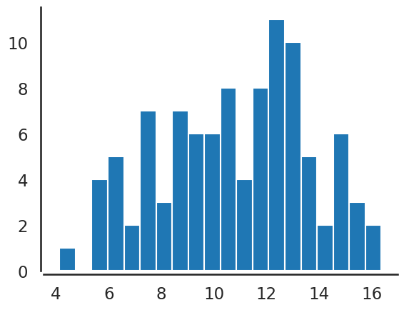
sigma = 3 # Note this is the std of our data
data = norm(10,sigma).rvs(100)

# hyperparameters on prior for mu
mu_prior = 8
sigma_prior = 1.5

plt.hist(data,bins=20)
sbn.despine(offset=3.)
plt.show()
PyMC#
Let’s use PyMC to model this:
This is the model statement describing priors and the likelihood.
Here, mu is defined as a stochastic variable (we want a chain of
sampled values for this variable) and we provide a prior distribution
and hyper-parameters for it. The likelihood function is chosen to be
Normal, with one parameter to be estimated (mu), and we use known
\(\sigma\) (denoted as sigma). Our “dependent variable” is given by
observed=data, where data is generated above and shown in the
histogram. In more formal terms, the code below sets up a
basic_model having the following form:
where \(\phi(.)\) is the standard normal pdf.
This code sets up the model (with name basic_model) but doesn’t sample from it:
import pymc as pm

with pm.Model() as basic_model:

    # Priors for unknown model parameters
    mu = pm.Normal('Mean of Data',mu_prior,sigma_prior)

    # Likelihood (sampling distribution) of observations
    data_in = pm.Normal('Y_obs', mu=mu, sigma=sigma, observed=data)
The following uses our PyMC model and proceeds with sampling. We will set starting values at MAP and use a Metropolis step method (which is Random Walk MH that we have studied so far).
chain_length = 10000

with basic_model:
    # obtain starting values via MAP
    startvals = pm.find_MAP(model=basic_model)
    print(startvals)
    # instantiate sampler
    step = pm.Metropolis()

    # draw posterior samples
    trace = pm.sample(chain_length, step=step, initvals=startvals, tune=1000,
                       return_inferencedata=True, progressbar=False)
{'Mean of Data': array(10.69594596)}
Multiprocess sampling (2 chains in 2 jobs)
Metropolis: [Mean of Data]
Sampling 2 chains for 1_000 tune and 10_000 draw iterations (2_000 + 20_000 draws total) took 2 seconds.
We recommend running at least 4 chains for robust computation of convergence diagnostics
A few things to note about this code
We will tune and burn-in our sampler using the first 1000 samples. Note the option
discard_tuned_samplesby default is set toTrue. Therefore our sampler is actually sampling 11,000 times but only returning 10,000.We are starting our chain using MAP. This may or may not be a good idea depending on your problem. If we don’t supply starting values,
PyMCmakes intelligent decisions about starting values.We are using random-walk Metropolis Hastings using the
Metropolis()step method. This method auto-tunes the proposal width and discards the samples during the tuning process (first 1000 samples).Note that the sampler automatically samples multiple independent chains (for Gelman-Rubin convergence criteria). By default 4 cores are sampled unless there are fewer processor cores available (in which case the number of samples is equal to the number of cores, but no less than 2).
In addition to having an easy way to setup and sample from a model
without having to write the accept/reject algorith, PyMC offers a
full suite of tools for visualizing and assessing the convergence
properties of your chain.
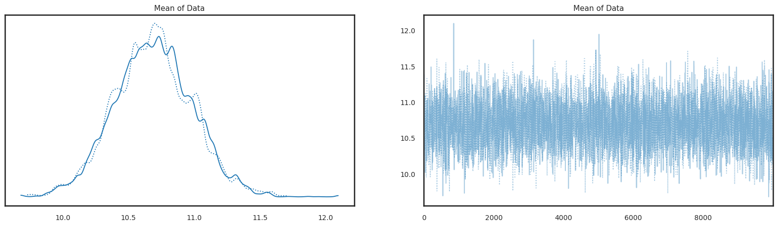
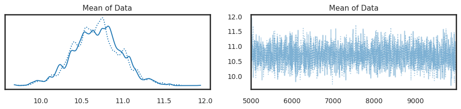
Visualize the traces. For each of the four chains:
pm.plot_trace(trace,figsize=(20,5));
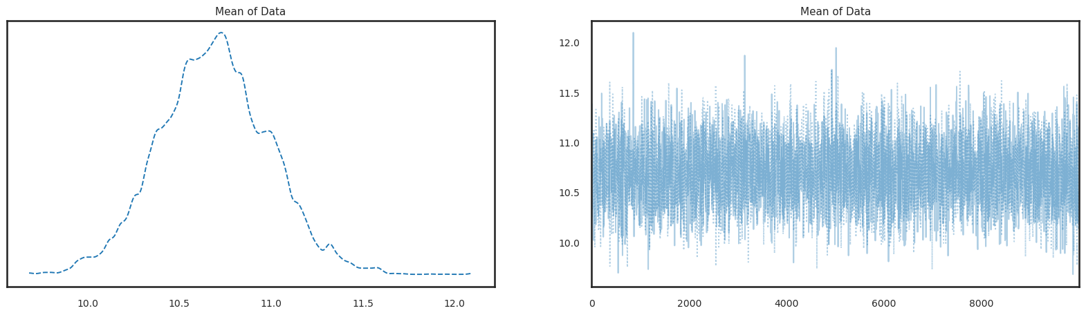
or we can combine all information for the histogram on the left panel (visualization of the posterior) across all chains
pm.plot_trace(trace, figsize=(20,5), combined=True);
Summarize the posterior. Note by default, this combines samples across all chains:
pm.summary(trace)
| mean | sd | hdi_3% | hdi_97% | mcse_mean | mcse_sd | ess_bulk | ess_tail | r_hat | |
|---|---|---|---|---|---|---|---|---|---|
| Mean of Data | 10.69 | 0.297 | 10.104 | 11.215 | 0.005 | 0.003 | 3783.0 | 4091.0 | 1.0 |
Note, that the summary has useful convergence criteria for each
parameter (r_hat) is the Gelman Rubin statistic, and the effective
sample size measures are given by ess_bulk and ess_tail.
Understanding the PyMC Results Object#
All the results are contained in the trace variable. Since in the
above pm3.sample call, we specified inference_data=True, this
returns and Arviz inference data. What you need to know about this
is that it is a data standard for multiple Bayesian software packages
and understanding the structure of this object is useful in numerous
ways.
First, notice that the object organizes information for our simple model around the following keys (identifiers):
trace.keys()
KeysView(Inference data with groups:
	> posterior
	> sample_stats
	> observed_data)
For our purposes, the posterior and sample_stats are the most
important items to focus on. Look inside the object to examine the
estimated mean inside the posterior:
trace.posterior
<xarray.Dataset>
Dimensions:       (chain: 2, draw: 10000)
Coordinates:
  * chain         (chain) int64 0 1
  * draw          (draw) int64 0 1 2 3 4 5 6 ... 9994 9995 9996 9997 9998 9999
Data variables:
    Mean of Data  (chain, draw) float64 10.78 10.78 10.78 ... 10.51 10.51 10.51
Attributes:
    created_at:                 2024-01-12T10:52:02.605841
    arviz_version:              0.17.0
    inference_library:          pymc
    inference_library_version:  5.10.3
    sampling_time:              2.3172712326049805
tuning_steps: 1000Further we can drill down to examine only the sampled Mean of Data
parameter:
trace.posterior['Mean of Data']
<xarray.DataArray 'Mean of Data' (chain: 2, draw: 10000)>
array([[10.78335751, 10.78335751, 10.78335751, ..., 10.31184733,
        10.31184733, 11.17041015],
       [10.66553476, 10.66553476, 10.86596014, ..., 10.5130954 ,
        10.5130954 , 10.5130954 ]])
Coordinates:
* chain (chain) int64 0 1
* draw (draw) int64 0 1 2 3 4 5 6 7 ... 9993 9994 9995 9996 9997 9998 9999Notice that the name each parameter tracked inside the posterior is
exactly as specified in the pymc model. If you want to extract
your samples and place them in a numpy array, use
trace_np = trace.posterior['Mean of Data'].to_numpy()
This trace has the following shape:
trace_np.shape
(2, 10000)
Where the first dimension is the number of chains, and the second is the number of samples per chain.
Selecting subsets of chains/samples from the Inference Data object#
Sometimes you want to
Only examine a single chain, or
Omit burn-in observations
Before running diagnostics or visualizing the results. The sel
method is useful in this regard. Suppose we only want to visualize a
single chain:
pm.plot_trace(trace.sel(chain=[0]));
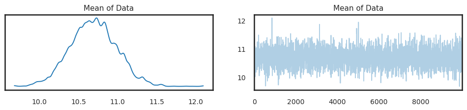
This performs a trace plot over only the first chain, rather than over all of them. One can also “drop” samples if you need longer burn-in:
keep_samples = [i for i in range(5000,10000)]
trace_burn_in = trace.sel(draw=keep_samples)
pm.plot_trace(trace_burn_in);
This shows a traceplot for the last 5000 samples for each chain (dropping the first 5000). Using similar techniques, we can also compute summaries only on these last 5000 samples:
pm.summary(trace_burn_in)
| mean | sd | hdi_3% | hdi_97% | mcse_mean | mcse_sd | ess_bulk | ess_tail | r_hat | |
|---|---|---|---|---|---|---|---|---|---|
| Mean of Data | 10.685 | 0.294 | 10.104 | 11.207 | 0.007 | 0.005 | 2013.0 | 2019.0 | 1.0 |
Diagnostics#
Many of the key diagnostics discussed in the previous chapter are
already included in the summary call:
pm.summary(trace)
| mean | sd | hdi_3% | hdi_97% | mcse_mean | mcse_sd | ess_bulk | ess_tail | r_hat | |
|---|---|---|---|---|---|---|---|---|---|
| Mean of Data | 10.69 | 0.297 | 10.104 | 11.215 | 0.005 | 0.003 | 3783.0 | 4091.0 | 1.0 |
Note that:
r_hatis the Gelman-Rubin statisticThe two effective sample size statistics (beginning with
ess) are as discussed in the prior chapterThe standard error of sampling is provided by
mcse_mean
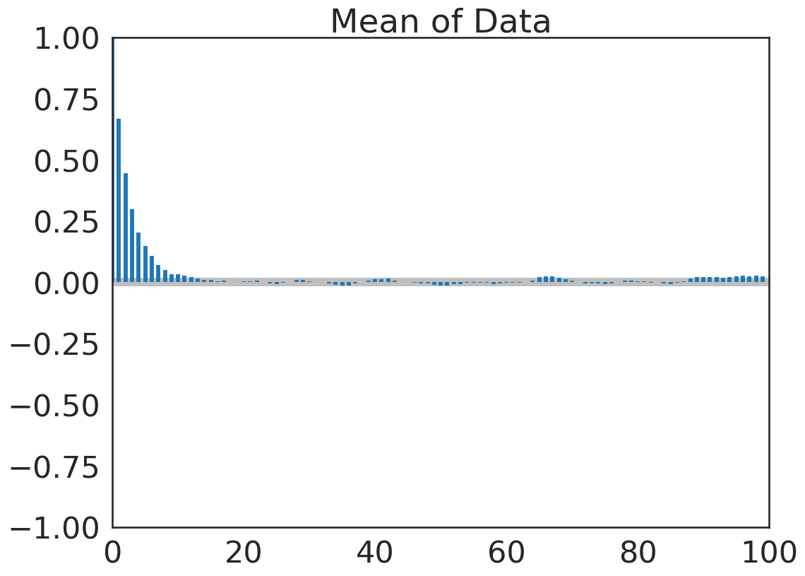
Autocorrelation Plots#
pm.plot_autocorr(trace,figsize=(17,5));
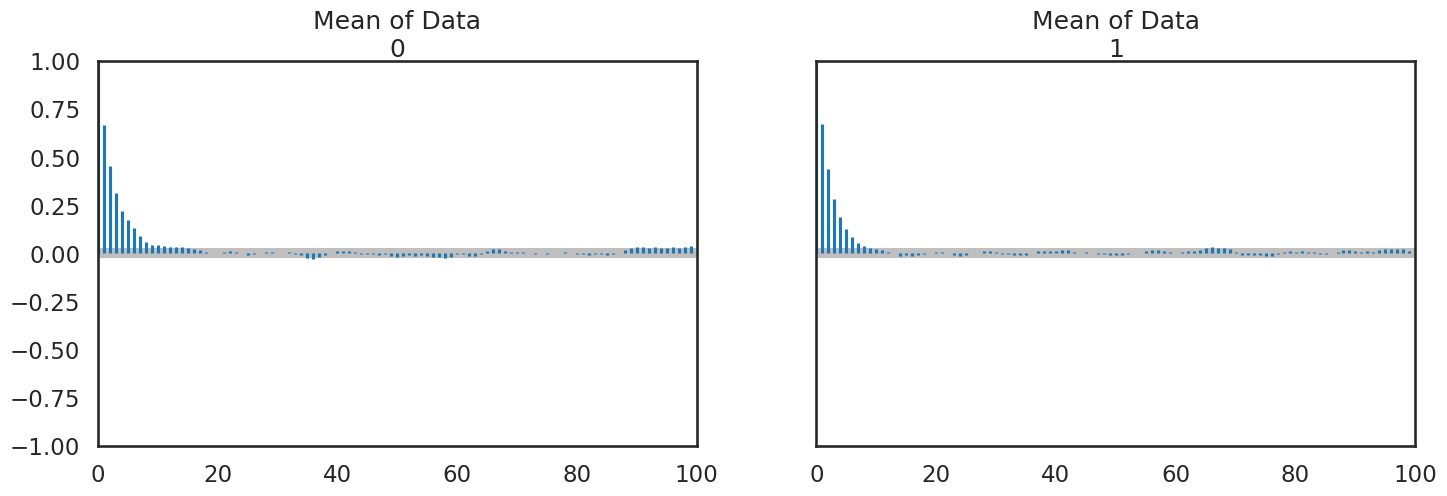
For me, this is better viewed as combined particularly after you examine the Gelman Rubin statistic and confirm convergence:
pm.plot_autocorr(trace, figsize=(12,9), combined=True);
Acceptance Rate#
The acceptance rate can also be computed from our trace object:
accept = trace.sample_stats.accepted.mean().to_numpy()
print("Acceptance Rate: ", accept.round(3))
Acceptance Rate: 0.329