from IPython.display import YouTubeVideo
import numpy as np
import pandas as pd
import matplotlib.pyplot as plt
import seaborn as sbn
from scipy.stats import norm, gamma, uniform
import pymc as pm
import arviz as az

import warnings
warnings.filterwarnings('ignore')

Step Methods for MCMC Sampling

In the previous chapter we saw that the sampling performance for the random-walk Metropolis Hastings algorithm (MWRW hereafter) led to low effective sample sizes, autocorrelation of some parameters, and convergence failure. The only strategy we had was to increase the number of samples to achieve good samples that meet the requirements of MCMC that we discussed previously.

This lecture builds on exciting recent work (last 15 years) that has led to massive improvements in sampling algorithms. These improvements mean that successful inference can proceed even with complicated models/posteriors with many fewer samples. Furthermore, these samples exhibit much less autocorrelation and rapid convergence. In my opinion the areas of Economics using Bayesian methods haven’t really exploited these innovations enough.

Note

These methods improve on the random walk Metropolis Hastings algorithm by generating less naiive proposals. The proposals will more efficiently explore the posterior space by using these improved step methods.

Here, I’ll briefly describe some of the step methods for producing a Monte Carlo Markov Chain. We have discussed in detail the random walk Metropolis Hastings sampler. We will briefly discuss in a bit more detail the following samplers:

1. Gibbs Samplers

2. Metropolis Hastings Samplers a. Random Walk Metropolis Hastings b. Differential Evolutionary Metropolis Hastings c. Adaptive Metropolis Hastings (we won’t cover) d. Independent Metropolis Hastings (we won’t cover) e. Slice Samplers and Other variants (we won’t cover)

The nitty-gritty details of the following two samplers are beyond the scope of the course, but I will try to give you a feel for how they improve on Metropolis Hastings and Gibbs methods because they are known to be a major improvement over any of the samplers listed above even for high dimensional models (lots of coefficients to estimate):

• Hamiltonian Monte Carlo Sampler (No U-turn Sampler, or NUTS)

• Affine Invariant Sampler (EMCEE) (we won’t cover)

An important point to consider about these methods is that Gibbs, most of the Metropolis Hastings samplers, and EMCEE are gradiant-free samplers. They do not require the calculation of the \(K\) dimenional slopes of the posterior. NUTS requires gradiant calculations. Recent innovations in scientific computing libraries (e.g. Jax, PyTensor, Tensorflow, PyTorch, autograd) means that auto differentiation is possible (the computer can rapidly assess the gradiant for ANY model you specify). This makes NUTS especially attractive.

This is a very fast moving topic, and a good place to stay up to date is on the Stan or PyMC github sites.

Gibbs Sampler

The Gibbs Sampler is a special case of the Random-Walk Metropolis Hastings algorithm and one worth knowing about in a bit of detail because many tutorials and discussions about MH (especially older ones) are entertwined with discussions on Gibbs sampling and it can be confusing for the uninitiated. Despite this being a special case of MH, it is worth seeing how it works in a bit of detail. The idea is to successively sample each \(\theta\) from its conditional distribution:

(4)\[\begin{align} \theta^{t+1}_1 \sim & f_1(\theta^{t+1}_1 \mid \theta^{t}_2,\theta^{t}_3,\ldots, \theta^{t}_k,\mathbf{y},\mathbf{x}) \\ \theta^{t+1}_2 \sim & f_2(\theta^{t+1}_2 \mid \theta^{t+1}_1,\theta^{t}_3,\ldots, \theta^{t}_k,\mathbf{y},\mathbf{x}) \\ \theta^{t+1}_3 \sim & f_3(\theta^{t+1}_3 \mid \theta^{t+1}_1,\theta^{t+1}_2,\ldots, \theta^{t}_k,\mathbf{y},\mathbf{x})\\ &\vdots \\ \theta^{t+1}_k \sim & f_k(\theta^{t+1}_k \mid \theta^{t+1}_1,\theta^{t+1}_2,\theta^{t+1}_3\ldots, \theta^{t+1}_{k-1},\mathbf{y},\mathbf{x}) \end{align}\]

where each parameter \(i\) has a conditional distribution function \(f_i\).

First consider this simple example, where our parameters to be estimate are \(\theta = [\mu,\sigma]\) and where we have flat priors:

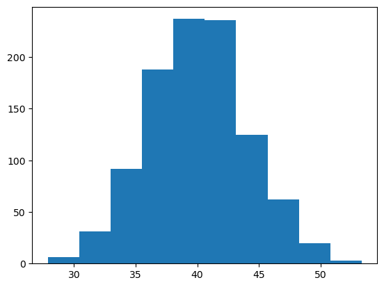
# data: construct toy data matrix
N = 1000
Y = norm(40,4).rvs(N)
plt.hist(Y);

When we employ a Gibbs Sampler, all samples are accepted (there are versions of the Gibbs Sampler that use a rejection based approach- not covered here). This is accomplished by choosing problems where the conditional distributions:

(5)\[\begin{align} f_\mu(\mu | \sigma, \mathbf{Y}) \\ f_\sigma(\sigma | \mu, \mathbf{Y}) \end{align}\]

are known and have closed form solutions. For example, if we have

(6)\[\begin{equation} f_\mu(\mu | \sigma, \mathbf{Y}) = \phi \left ( \frac{\mathbf{Y} - \mu}{\sigma} \right ) \end{equation}\]

that is, Y is distributed normal with mean \(\mu\) and standard deviation \(\sigma\), then it can be shown that

(7)\[\begin{equation} f_\sigma \left(\sigma^2 | \mu, \mathbf{Y}\right ) = InverseGamma(k,s) \end{equation}\]

where \(k\) and \(s\), the shape and scale parameters for the Inverse Gamma Distribution are

(8)\[\begin{align} k &= \frac{n}{2} \\ s &= \left (\frac{(Y-\mu)^2}{2} \right )^{-1} \end{align}\]

The Gibbs Sampler then proceeds as follows:

1. Start the sampler at an arbitrary starting value for \(\theta\). In my code below, I start the Gibbs sampler at \(\theta_0 = [\mu_0=30,\sigma_0=3]\).

2. Draw the next (always accepted) value of \(\sigma_t\) by:

   1. Draw random variate from a gamma distribution, \(\Gamma(k,s) = \Gamma \left ( \frac{n}{2},\left (\frac{(Y-\mu_{t-1})^2}{2} \right )^{-1} \right )\) and denote as \(g\)

   2. Define \(var_t = \frac{1}{g}\)

3. Draw the next (always accepted) value of \(\mu_t\) by:

   1. Draw a normal random variate having mean \(\bar{Y}\) and standard deviation \(\sqrt{\frac{var_t}{n}}\) and denote as \(\mu_t\).

4. Store the values \([\mu_t,\sqrt{var_t}]\) as the next sampled values for \(\mu\) and \(\sigma\).

Important thing to note about this process:

1. Gibbs sampling depends on our ability to analytically solve for conditional distributions

2. This involves derivations in mathematical statistics

3. Once we have these closed form solutions, we can accept every sampled draw

Here is an example of Gibbs sampling in code, so you can see how it proceeds:

chain_len = 10000
burnin = 1000

# store chains here:
mu_chain_gibbs =np.zeros((chain_len+burnin,1)) 
sigma_chain_gibbs = np.zeros(mu_chain_gibbs.shape)

# starting guesses for mu
mu_old = 20

for i in np.arange(chain_len+burnin):
    gamma_new = gamma(len(Y)/2,scale=1/np.sum(((Y-mu_old)**2)/2)).rvs()
    var_new = 1/gamma_new
    mu_new = norm(np.mean(Y), np.sqrt(var_new/len(Y))).rvs(1)
    mu_chain_gibbs[i] = mu_new
    sigma_chain_gibbs[i] = np.sqrt(var_new)
    # reset old values
    mu_old, var_old = mu_new, var_new

Now examine the output:

# convert to pandas dataframe
chain_gibbs = pd.DataFrame(np.append(mu_chain_gibbs, sigma_chain_gibbs, 1),
                           columns=['mean','std'])
# calculate summary statistics post burn-in
chain_gibbs.loc[burnin:].describe(percentiles=[.025, .5, .975])

	mean	std
count	10000.000000	10000.000000
mean	40.057838	3.978664
std	0.124267	0.088448
min	39.597146	3.676352
2.5%	39.812753	3.812778
50%	40.059440	3.975518
97.5%	40.303345	4.158292
max	40.474121	4.316474

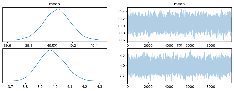
The trace looks like this:

plot_gibbs = chain_gibbs.loc[burnin:]

# convert to arviz inference_data for
# plotting with pm
inf_data = az.from_dict(
    posterior={
        "mean": plot_gibbs['mean'].values,
        "std": plot_gibbs['std'].values
    }
)

pm.plot_trace(inf_data);

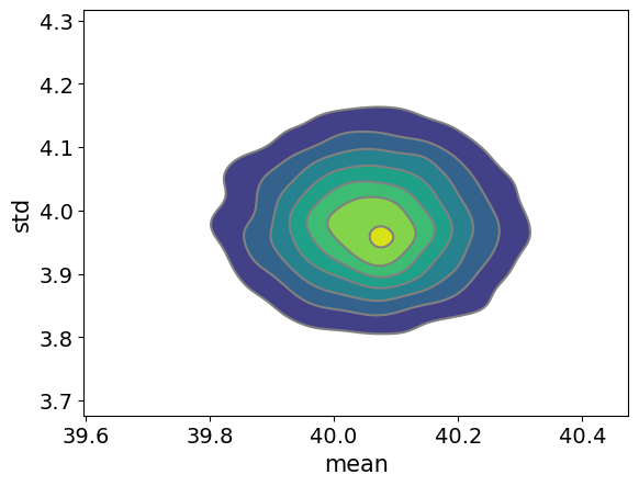
Here is a plot of the posterior:

pm.plot_pair(inf_data, kind='kde');

Because users have to so carefully choose conditional distributions for Gibbs sampling, PyMC does not include a Gibbs sampler (it does have a special Gibbs within MH for categorical variables).

In addition to the MHRW, the Gibbs Sampler was the predominant sampling method early on in applied Bayesian statistics because it has real advantages over MHRW for problems having solvable conditional distributions since it accepts every sample and can be more efficient (less computing time to reach convergence and inference).

Despite this, both the Gibbs Sampler and the MH Random Walk Sampler are less than ideal for situations where we have

1. high dimensional problems (many parameters), and/or

2. high correlation amongst parameters

For the empirical excercises below, we’ll be reusing the Tobias and Koop dataset and estimate as Pooled OLS (with the associated caveats outlined in the previous chapter). Loading the data:

tobias_koop = pd.read_stata('https://rlhick.people.wm.edu/econ407/data/tobias_koop.dta')
tobias_koop.head()

	id	educ	ln_wage	pexp	time	ability	meduc	feduc	broken_home	siblings	pexp2
0	1.0	13.0	1.82	1.0	0.0	1.0	12.0	12.0	0.0	1.0	1.0
1	1.0	18.0	3.29	3.0	7.0	1.0	12.0	12.0	0.0	1.0	9.0
2	1.0	18.0	3.21	5.0	9.0	1.0	12.0	12.0	0.0	1.0	25.0
3	1.0	18.0	3.06	6.0	10.0	1.0	12.0	12.0	0.0	1.0	36.0
4	2.0	15.0	2.14	4.0	6.0	1.5	12.0	12.0	0.0	1.0	16.0

For all of the models explored here, we’ll be estimating the OLS model discussed in the previous chapter:

with pm.Model() as ols_model:
    
    # priors
    b0 = pm.Normal('constant', mu=0., sigma=10.)
    b1 = pm.Normal('educ', mu=0., sigma=10.)
    b2 = pm.Normal('pexp', mu=0., sigma=10.)
    b3 = pm.Normal('broken_home', mu=0., sigma=10.)
    sigma = pm.Uniform('sigma', lower=.1, upper=10.)

    # yhat (or the mean for each i's likelihood contrib)
    mu_i = b0 + b1 * tobias_koop.educ + b2 * tobias_koop.pexp +\
                b3 * tobias_koop.broken_home
        
    # likelihood
    like = pm.Normal('likelihood', mu=mu_i, sigma=sigma, 
                      observed = tobias_koop.ln_wage)

One very useful property of our ols_model is that we have defined it independently of the sampling step method, so we can “run” the model using any valid PyMC step method. Note two things:

1. see the previous chapter if you are unclear about what the code above is doing as we motivate the model and code there

2. we don’t include the predicted wage or elasticity calculations in our trace, but could

Step Methods

We will re-explore the MHRW step method applied to our model and will introduce the Differential Evolutionary Metropolis Hastings step method. Then we will discuss in some detail a few other widely used-samplers.

MHRW

We have already seen the MHRW step method at work in PyMC, but for comparison purposes, let’s reproduce the model from last time:

Sampling from the posterior for the model is accomplished using

with ols_model:
    step = pm.Metropolis()
    start = pm.find_MAP()
    samples_mhrw = pm.sample(1000, step=step, tune=1000, initvals=start, 
                       return_inferencedata=True, progressbar=False)

100.00% [72/72 00:00<00:00 logp = -12,445, ||grad|| = 80.824]

Multiprocess sampling (2 chains in 2 jobs)

CompoundStep

>Metropolis: [constant]

>Metropolis: [educ]

>Metropolis: [pexp]

>Metropolis: [broken_home]

>Metropolis: [sigma]

Sampling 2 chains for 1_000 tune and 1_000 draw iterations (2_000 + 2_000 draws total) took 3 seconds.

We recommend running at least 4 chains for robust computation of convergence diagnostics

Note, we are intentionally curtailing sampling at 1000 samples with 1000 burn-in and tuning samples, for comparing the relative performance of the other samplers in this lecture. We know this fails to achieve convergence based on Gelman-Rubin’s r_hat:

pm.summary(samples_mhrw)

	mean	sd	hdi_3%	hdi_97%	mcse_mean	mcse_sd	ess_bulk	ess_tail	r_hat
constant	0.819	0.022	0.789	0.858	0.014	0.011	3.0	16.0	2.18
educ	0.093	0.002	0.090	0.095	0.001	0.001	3.0	17.0	2.10
pexp	0.037	0.001	0.036	0.039	0.000	0.000	19.0	23.0	1.09
broken_home	-0.055	0.010	-0.076	-0.039	0.001	0.001	189.0	154.0	1.01
sigma	0.484	0.003	0.480	0.489	0.000	0.000	186.0	248.0	1.01

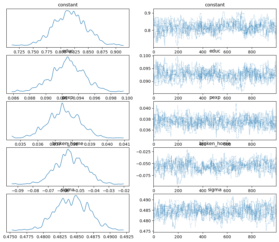
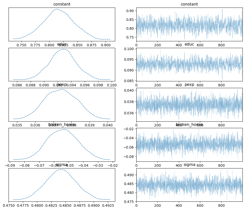
And the trace plot:

pm.plot_trace(samples_mhrw, combined=True);

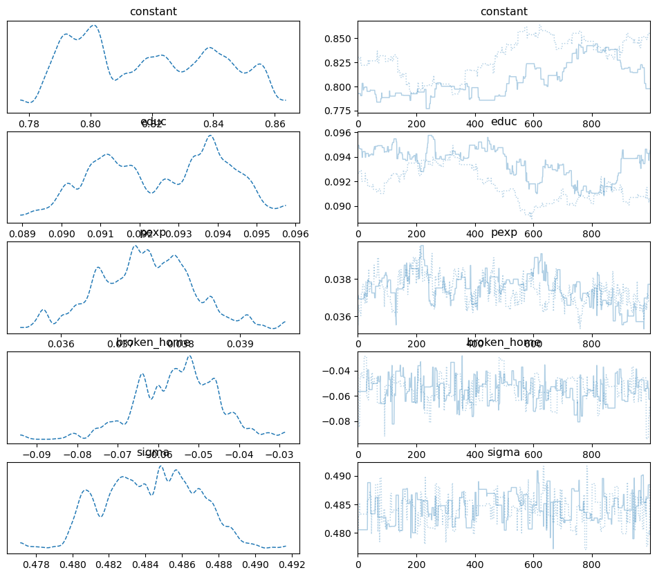
Note, you can see the autocorrelation in these plots as the trace for each separate chain moves in predictable ways.

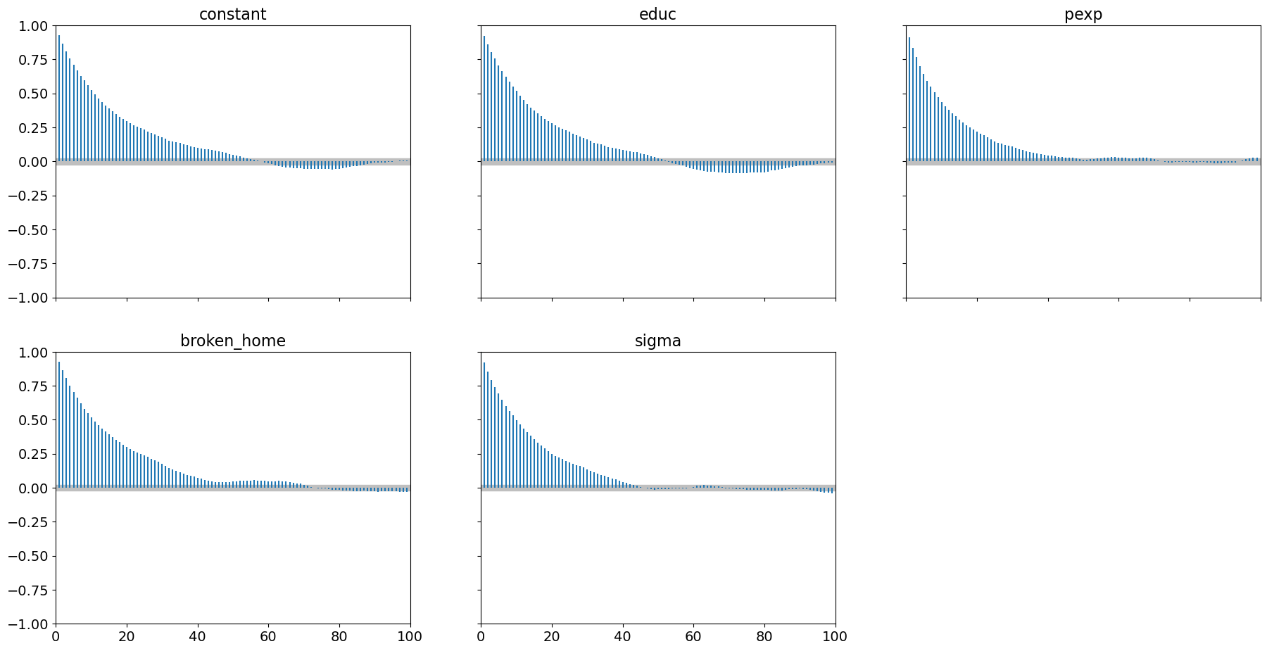
This is reinforced by the autocorrelation plot:

pm.plot_autocorr(samples_mhrw, combined=True);

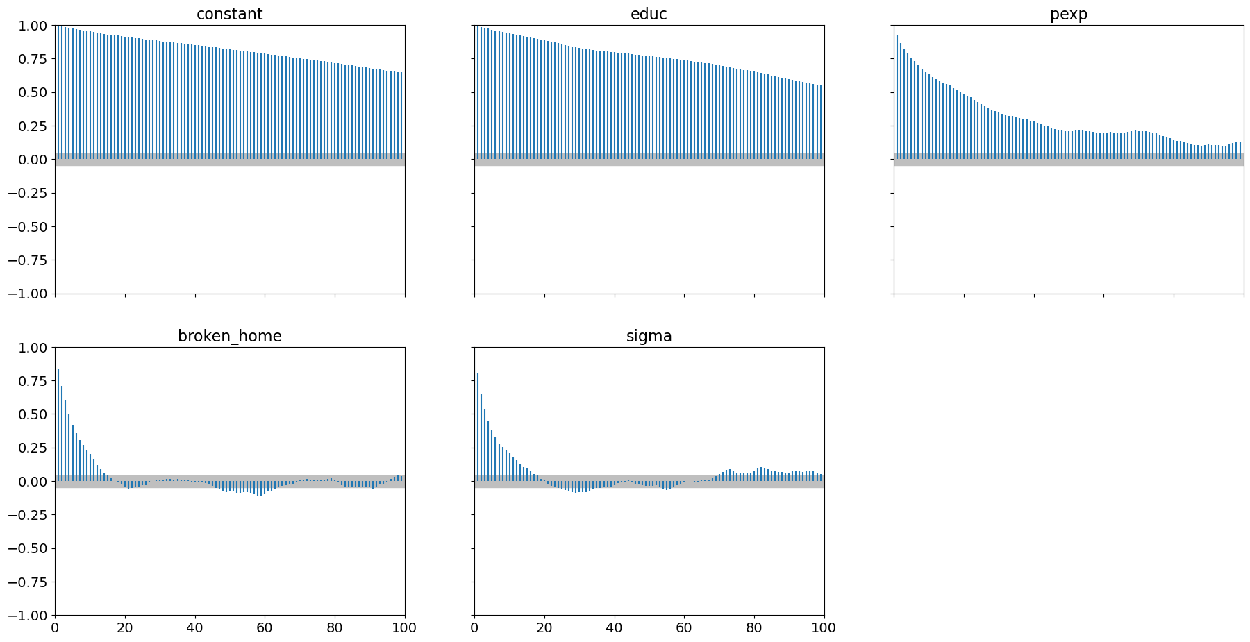
It is evident that 2000 samples (with 1000 of those as burn-in) is woefully inadequate.

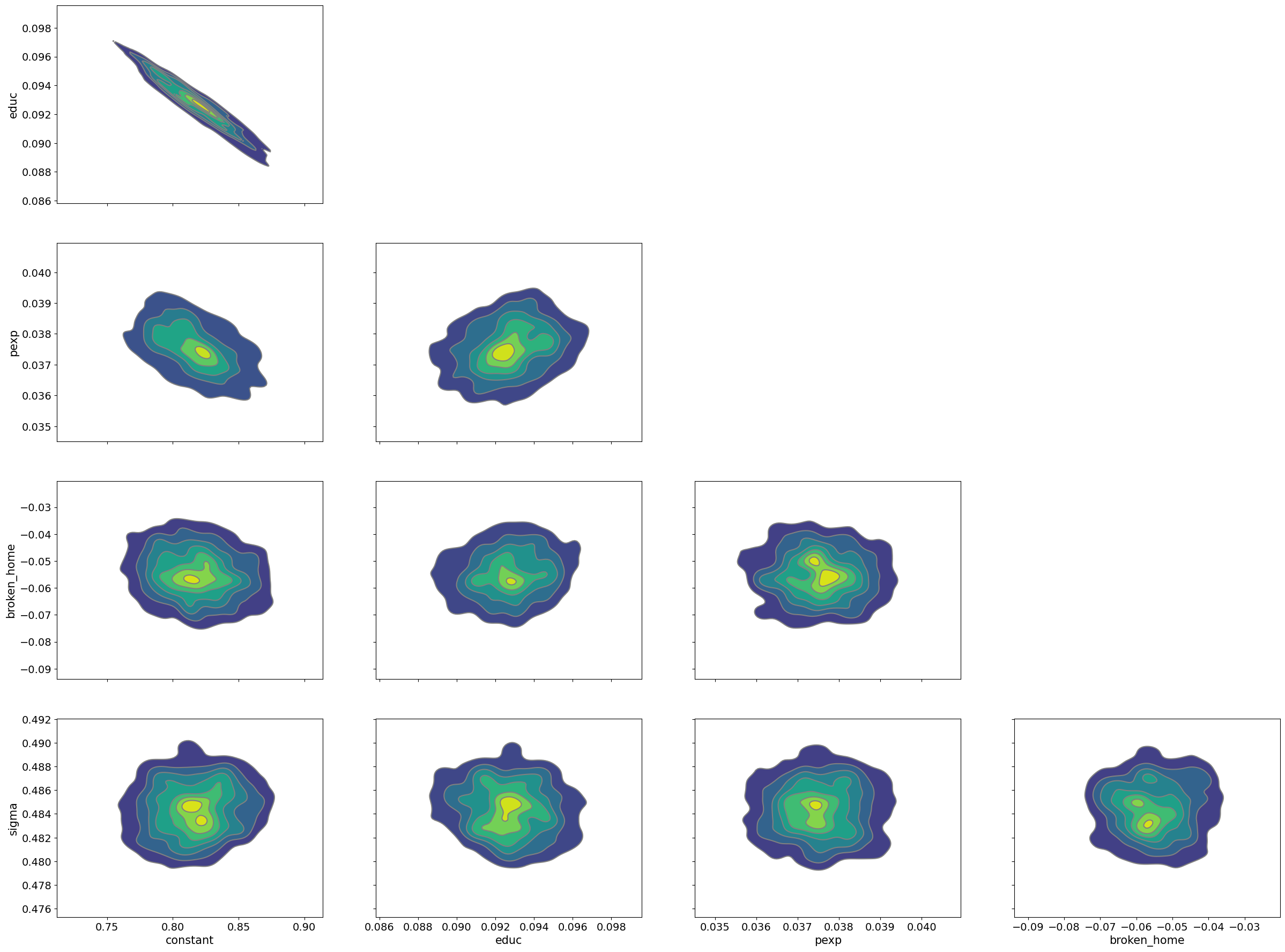
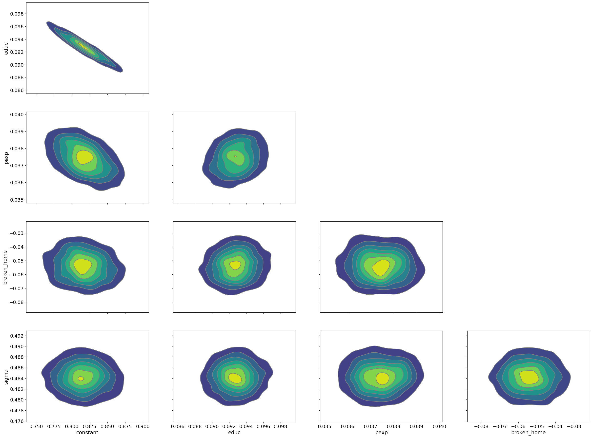
Finally, it is worth examining the pair plot to see where potential correlations amongst parameters might be causing MHRW to fail:

pm.plot_pair(samples_mhrw, kind='kde');

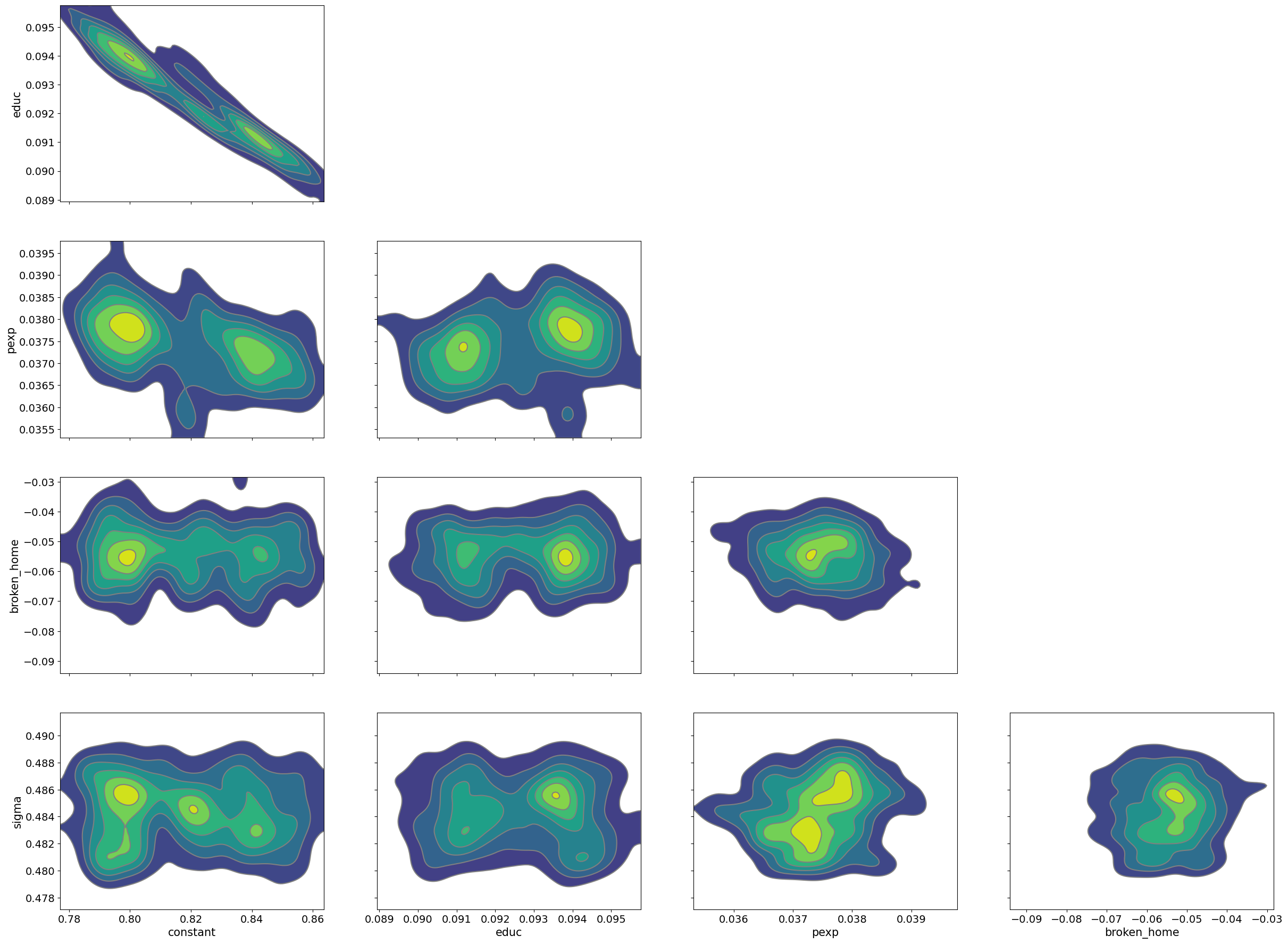
Note that in particular, education and the model constant have high degrees of correlation. This means that as a pair parameter vectors tend to be accepted/rejected as the parameter space is being explored. This is being driven by the posterior and is not a warning sign for our model, however, MHRW is not well suited for these types of correlations.

Differential Evolutionary Metropolis Hastings

MHRW has been modified to improve on the random walk aspect of generating proposals. One such step method is the Differential Evolutionary Metropolis-Hastings algorithm.

Our posterior draws from Metropolis-Hastings Random Walk shows that

1. We treat each parameter as independent

2. Yet in the samples in the posterior, there are significant covariances

Idea: generate multiple chains (this method calls each chain a population) and for each proposal step randomly sample points in other chains to calculate a direction and distance for the next proposal. In short, the step method cross-sample for more efficient search of the posterior.

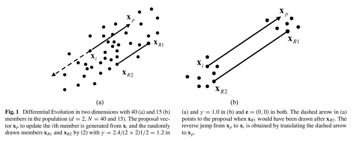
Fig. 7 How Differential Evolutionary MH Works

The paper describing this in more detail is available on our google drive site here. For comparisons to later step methods it is useful to note that this method does not require gradiants.

With PyMC it is quite easy to implement, noting that the more chains we construct the better (note, this may run slow or fail to run on your machine), so we set chains=8 (you want to have lots of chains for improving the efficiency of the sampler, here we set chains=8 for running on the jupyterhub server):

with ols_model:
    # instantiate sampler
    step = pm.DEMetropolis() 

    # draw posterior samples
    samples_mhde = pm.sample(1000, tune=1000, initvals=start,
                          step=step, progressbar=False, 
                          chains=8, return_inferencedata=True) 

Population sampling (8 chains)

DEMetropolis: [constant, educ, pexp, broken_home, sigma]

Attempting to parallelize chains to all cores. You can turn this off with `pm.sample(cores=1)`.

Sampling 8 chains for 1_000 tune and 1_000 draw iterations (8_000 + 8_000 draws total) took 6 seconds.

The rhat statistic is larger than 1.01 for some parameters. This indicates problems during sampling. See https://arxiv.org/abs/1903.08008 for details

The effective sample size per chain is smaller than 100 for some parameters.  A higher number is needed for reliable rhat and ess computation. See https://arxiv.org/abs/1903.08008 for details

Here is the summary of the trace:

# note, randomly choose 4 chains only for summary/convergence 
# checks for "fair" comparison
chains = np.random.choice(range(8), 4)
pm.summary(samples_mhde.sel(chain=chains))

	mean	sd	hdi_3%	hdi_97%	mcse_mean	mcse_sd	ess_bulk	ess_tail	r_hat
constant	0.817	0.029	0.765	0.869	0.002	0.002	138.0	278.0	1.04
educ	0.093	0.002	0.089	0.096	0.000	0.000	142.0	234.0	1.04
pexp	0.038	0.001	0.036	0.039	0.000	0.000	167.0	270.0	1.02
broken_home	-0.056	0.010	-0.073	-0.038	0.001	0.001	129.0	245.0	1.02
sigma	0.484	0.003	0.480	0.489	0.000	0.000	162.0	242.0	1.02

Notice, we have convergence whereas with mhrw we did not, for any four randomly selected chains (for perhaps a fairer comparison to the mhrw results above). Since we have 8 chains, we should focus on the summary from all of them:

pm.summary(samples_mhde)

	mean	sd	hdi_3%	hdi_97%	mcse_mean	mcse_sd	ess_bulk	ess_tail	r_hat
constant	0.817	0.029	0.760	0.867	0.002	0.001	258.0	417.0	1.03
educ	0.093	0.002	0.089	0.096	0.000	0.000	272.0	326.0	1.02
pexp	0.038	0.001	0.036	0.039	0.000	0.000	337.0	423.0	1.02
broken_home	-0.055	0.010	-0.074	-0.038	0.001	0.000	241.0	453.0	1.04
sigma	0.484	0.003	0.480	0.489	0.000	0.000	303.0	536.0	1.02

And the trace plot:

pm.plot_trace(samples_mhde, combined=True);

Compared to mhrw we have much better mixing occuring and convergence is achieved. This is reinforced by the autocorrelation plots:

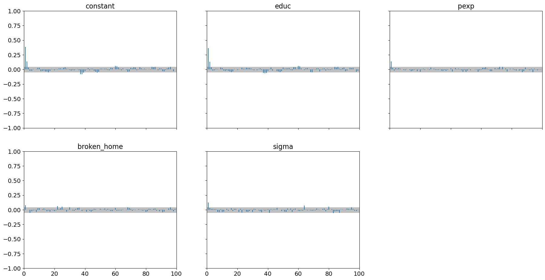
pm.plot_autocorr(samples_mhde, combined=True);

For this step method, convergence performance for these 2000 samples is much better than Metropolis Hastings.

Finally, it is worth examining the pair plot to see where potential correlations amongst parameters and how this step method handles it:

pm.plot_pair(samples_mhde, kind='kde');

Hamiltonian Monte Carlo and the No U-turn Sampler

Hamiltonian Monte Carlo was developed initially in the field of particle physics for simulating the movement of molecules in three dimensions. It is trivially extended to \(k\) dimensions (our parameter space). This step method adds an auxiliary parameter for each model parameter and therefore doubles the parameter space in a way that actually makes the exploration of the posterior more efficient. These auxiliary parameters (nuisance parameters) are discarded after estimation. Our original model parameters (helps us to define potential energy which is the posterior probability) and these auxiliary parameters (helps us define kinetic energy), which aid in a more efficient exploration of the parameter space. An excellent discussion of Hamiltonian Monte Carlo is here and the paper extending Hamiltonian Monte Carlo to the No U-Turn Sampler is here. These don’t make for light reading and are not required for this course.

The idea: rather than blindly stumbling around the posterior, use the posterior gradiant to skate around the gradiant contour. As you skate closer to a drop-off (gradiant is steep and probability is lower), potential energy decreases and kinetic energy increases (since energy is always conserved). When this happens the skater usually is turned back uphill and pushed from the precipice and skates on along a posterior likelihood contour. The No U-Turn sampler keeps skating until the skater tries to turn back towards the original point.

One trick to applying this method is to ensure that proposals lead to accepted samples that satisfy the Ergodic Theorem. The papers above go into that topic.

Using PyMC, we can implement NUTS quite easily as it is the default step method (NUTs is auto-assigned for many types of posteriors) as:

with ols_model:
    # declare sampler here. Comment out for auto assignment
    step = pm.NUTS() 
    
    # draw posterior samples
    samples_nuts = pm.sample(1000, tune=1000, initvals=start, step=step,
                              return_inferencedata=True)

Multiprocess sampling (2 chains in 2 jobs)

NUTS: [constant, educ, pexp, broken_home, sigma]

100.00% [4000/4000 00:21<00:00 Sampling 2 chains, 0 divergences]

Sampling 2 chains for 1_000 tune and 1_000 draw iterations (2_000 + 2_000 draws total) took 22 seconds.

We recommend running at least 4 chains for robust computation of convergence diagnostics

Summarizing the chain, we see Gelman-Rubin r_hat scores very close to 1 and very high effective sample sizes:

pm.summary(samples_nuts)

	mean	sd	hdi_3%	hdi_97%	mcse_mean	mcse_sd	ess_bulk	ess_tail	r_hat
constant	0.816	0.027	0.766	0.867	0.001	0.001	953.0	808.0	1.0
educ	0.093	0.002	0.089	0.097	0.000	0.000	973.0	1016.0	1.0
pexp	0.037	0.001	0.036	0.039	0.000	0.000	1533.0	1266.0	1.0
broken_home	-0.054	0.010	-0.072	-0.035	0.000	0.000	1732.0	1301.0	1.0
sigma	0.484	0.003	0.480	0.489	0.000	0.000	1449.0	1141.0	1.0

with the trace plot:

pm.plot_trace(samples_nuts, combined=True);

with minimal autocorrelation:

pm.plot_autocorr(samples_nuts, combined=True);

We see it does a superb job with highly correlated parameters:

pm.plot_pair(samples_nuts, kind='kde');

For many types of problems, NUTS is the best step method. NUTS is a gradiant-based sampler and it uses a program called pytensor to provide auto differentiation: for any posterior you define. This allows PyMC to rapidly calculate gradiants without manually having to program them in this blog post describes in more detail what auto differentiation is.

A caveat to NUTS as implemented in PyMC:

NUTS uses a package called PyTensor (totally in the background) for compiling your model into faster code and providing gradiants. While that is nice, sometimes the error messages you might get are less than illuminating.

Sampler Summary

One way of seeing sampling efficiency is to look at only 1 chain for each method and plot the trace. This provides a quick visual inspection of how well a sampler is exploring the posterior. We do this below for the education parameter (noting that arviz doesn’t provide a mechanism for overlaying traceplots):

# extract a single chain from each method to a numpy array

plot_samples = [i.posterior.sel(chain=[0])['educ'].to_numpy().flatten() for i in\
                [samples_mhrw, samples_mhde, samples_nuts]]
sample_id = np.arange(1000)

Having extracted the data, let’s plot it:

plt.figure(figsize=(13,8))
plt.plot(sample_id, plot_samples[1], label = 'MHDE', lw = .5)
plt.plot(sample_id, plot_samples[2], label = 'NUTS', lw = .5)
plt.plot(sample_id, plot_samples[0], label = 'MHRW', lw = 1.75)
plt.title('Comparing Posterior Exploration for Various Step Methods')
plt.legend()
plt.show();

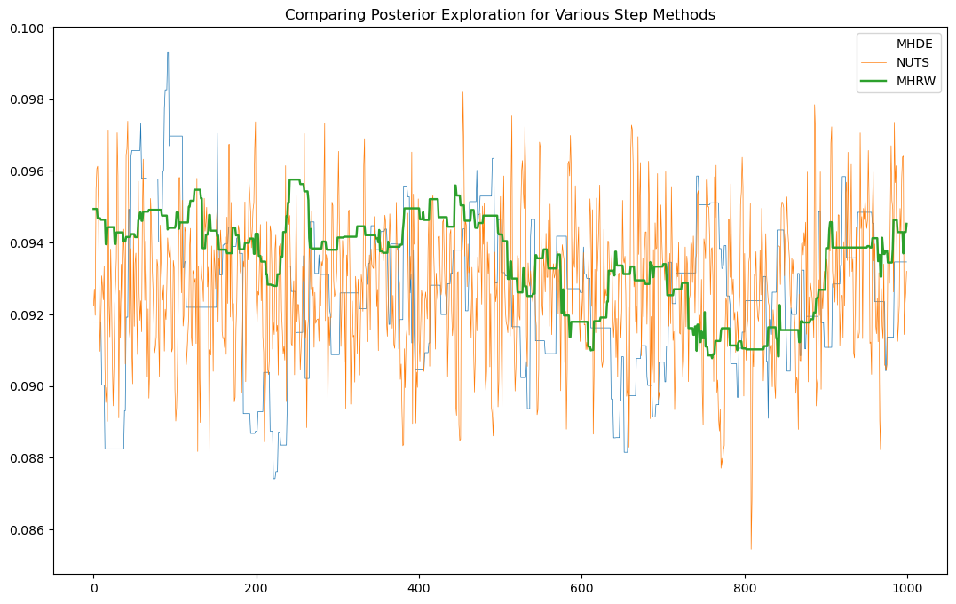
Further visualizations of the main contenders (NUTs and EMCEE) show the stark difference for how poor the performance of MHRW is.

For “difficult” posteriors:

• MHRW vs EMCEE (somewhat like Differential Evolutionary Metropolis)

YouTubeVideo('yow7Ol88DRk')

• MHRW vs NUTS

YouTubeVideo('Vv3f0QNWvWQ')

And for the Koop and Tobias data and the model outlined in this chapter, a comparison of MHRW, Differential Evolutionary MH, and NUTS focusing on two highly correlated parameters:

YouTubeVideo('Qv3u71UoPJU')

A few points are in order. NUTS is the “best” step method for a variety of settings. NUTS however can’t be used for discrete (or categorical) random variables, since gradiants are required. PyMC offers compound step methods which will sample continuous random variables using NUTS and discrete random variables using some form of Metropolis-Hastings. If you don’t specify step, PyMC has good heuristics for choosing the correct step method for your problem.

The two step methods requiring many chains (MHDE and EMCEE) will outperform NUTS for multimodel distributions or difficult posteriors. However, these often require multiple chains per parameter for proper mixing, which may not be practical for problems with large numbers of parameters (e.g. a 100 parameter problem might require 400 or more sampled chains). However, recent trends in GPU hardware and software allows for massive parralelization of sampling which will make the applicability of these step methods more widely used. PyMC also offers better access to GPU modeling with no (or little) change in code.

We have examined a few samplers (really these are alternative ways of generating proposals) that will be vastly superior to MH Random Walk in virtually all situations. This website while possibly outdated shows the many samplers that are out there and discusses their strength and weaknesses.

For the ones we considered, here is a summary table

Sampler	Acceptance Rate	Applications	Gradiant Required?	Final Grade
MH-RW	20-50%	High Numbers of Parameters and Discrete Distributions	No	D
MH-DE	44% for one parameter, 23.4% for five or more parameters	Good even with high number of parameters but need sufficient numbers of populations	No	B+
NUTS	80%	Excellent for any problem even high numbers of parameters if gradiants exist	Yes	A
EMCEE	44% for one parameter, 23.4% for five or more parameters	Good even with high number of parameters but requires at least 2 walkers per parameter	No	B+