import pandas as pd
import statsmodels as sm
import statsmodels.formula.api as smf
import pymc as pm
import numpy as np

Ordinary least squares using PyMC

Recall the ordinary least squares model you might be familiar with from a previous statistics or econometrics class. We are interested in estimating the parameter vector \(\beta\) from the following population regression function:

\[ \mathbf{y = x \beta + \epsilon} \]

where \(\mathbf{y}\) and \(\mathbf{\epsilon}\) are each \(N \times 1\) vectors of independent (outcome) and unobservable random variables. The \(N \times K\) matrix \(\mathbf{x}\) are the non-random (assumed for this notebook) independent variables (sometimes referred to as covariates). The least squares approach yields the “ols” estimator

\[ \mathbf{b} = \mathbf{{x'x}^{-1} x'y} \]

The frequentist approach performs inference based on the variance covariance matrix of \(\mathbf{b}\) which is estimated as

\[ cov(\mathbf{b}) = \hat{\sigma}^2 \left( \mathbf{x'x} \right)^{-1} \]

where \(\hat{\sigma}^2 = \frac{(\mathbf{y-xb})'(\mathbf{y-xb})}{N-K}\)

The square root of the diagonal of this matrix yields standard errors for estimated coefficients as reported in programs like Stata. These standard errors are used for inference related questions.

The Bayesian approach to OLS takes a different approach. Consider the model

\[\begin{split} \begin{align} \sigma &\sim Uniform(a=.01, b=10) \nonumber \\ \mathbf{\beta}_k &\sim N(\mu_b = 0, \sigma_b = 10) \text{ } \forall k \in K \nonumber\\ \mathbf{y} &\sim N(\mathbf{x\beta}, \sigma^2 I) \nonumber \end{align} \end{split}\]

We can setup the likelihood and priors for getting information about the posterior. Assembling the pieces,

1. Likelihood:

   \[ prob(\mathbf{y}| \mathbf{x}, \mathbf{\beta}, \mathbf{\sigma}) = \prod_{i=1}^N \frac{1}{\sqrt{2\pi\sigma^2}} e^\frac{(y_i-\mathbf{x}_i \mathbf{b})^2}{2\sigma^2} \]

2. Prior on \(\sigma\):

   \[ prob(\sigma | a=0.01, b=10) = \frac{1}{(10 - .01)} \text{ for } .01 \le \sigma \le 10 \text{, 0 otherwise} \]

3. Prior on \(\mathbf{\beta}\)

   \[ prob(\mathbf{b} | \mu_b = 0, \sigma_b = 10) = \prod_{k = 1}^{K} \frac{1}{\sqrt{2\pi \sigma^2_b}} e ^ {\frac{b_k - \mu_b}{2\sigma^2_b}} \]

Let \(\theta\) be the vector of all unknown parameters, \(\begin{bmatrix} \beta_1 \\ \vdots \\ \beta_k \\ \vdots \\ \beta_K \\ \sigma \end{bmatrix}\). Then the posterior is proportional to

\[ p(\theta | \mathbf{y}, \mathbf{x}, a, b, \mu_b, \sigma_b) \propto prob(\mathbf{y}| \mathbf{x}, \mathbf{\beta}, \mathbf{\sigma}) \times prob(\sigma | \alpha_l, \alpha_u) \times prob(\mathbf{b} | \mu_b = 0, \sigma_b = 10) \]

An example

We will use the Tobias and Koop dataset for this excercise. We’ll estimate a simple model using frequentist and Bayesian methods. This dataset has the following fields:

Variable	Definition
id	person id, ranging from 1 to 2,178
educ	education (years)
ln_wage	log of hourly wage
pexp	potential experience
time	time trend
ability	ability
meduc	mother’s education (years)
feduc	father’s education
broken_home	dummy variable for residence in a broken home
siblings	number of siblings
pexp2	squared potential experience

tobias_koop = pd.read_stata('https://rlhick.people.wm.edu/econ407/data/tobias_koop.dta')
tobias_koop.head()

	id	educ	ln_wage	pexp	time	ability	meduc	feduc	broken_home	siblings	pexp2
0	1.0	13.0	1.82	1.0	0.0	1.0	12.0	12.0	0.0	1.0	1.0
1	1.0	18.0	3.29	3.0	7.0	1.0	12.0	12.0	0.0	1.0	9.0
2	1.0	18.0	3.21	5.0	9.0	1.0	12.0	12.0	0.0	1.0	25.0
3	1.0	18.0	3.06	6.0	10.0	1.0	12.0	12.0	0.0	1.0	36.0
4	2.0	15.0	2.14	4.0	6.0	1.5	12.0	12.0	0.0	1.0	16.0

Note, that this is a panel dataset having the following time periods:

tobias_koop.time.value_counts()

time
12.0    1570
11.0    1535
10.0    1520
13.0    1517
14.0    1499
9.0     1443
8.0     1398
7.0     1284
6.0     1248
5.0     1093
4.0     1034
3.0      964
2.0      745
1.0      615
0.0      454
Name: count, dtype: int64

For purposes of this lecture we will ignore the panel aspects of this dataset and estimate an ordinary least squares model. Furthermore, due to memory constraints that students may encounter on jupyterhub for some of the features below, we will restrict our sample to time==4 (1983). In general we don’t recommend omitting data like this, but do it here for the aforementioned reasons. Reducing the data:

print("Records in original dataset: ", tobias_koop.shape[0])
tobias_koop = tobias_koop[tobias_koop.time == 4]
print("Records in reduced dataset: ", tobias_koop.shape[0])

Records in original dataset:  17919
Records in reduced dataset:  1034

Let’s estimate a simple wage model:

\[ ln\_wage_i = \beta_0 + \beta_1 educ + \beta_2 pexp + \beta_3 broken\_home_i + \epsilon_i \]

Using statsmodels, we have

res = smf.ols(formula='ln_wage ~ educ + pexp + broken_home', 
              data=tobias_koop).fit()
print(res.summary())

                            OLS Regression Results                            
==============================================================================
Dep. Variable:                ln_wage   R-squared:                       0.142
Model:                            OLS   Adj. R-squared:                  0.140
Method:                 Least Squares   F-statistic:                     57.04
Date:                Fri, 12 Jan 2024   Prob (F-statistic):           4.09e-34
Time:                        10:52:15   Log-Likelihood:                -598.31
No. Observations:                1034   AIC:                             1205.
Df Residuals:                    1030   BIC:                             1224.
Df Model:                           3                                         
Covariance Type:            nonrobust                                         
===============================================================================
                  coef    std err          t      P>|t|      [0.025      0.975]
-------------------------------------------------------------------------------
Intercept       0.6789      0.133      5.101      0.000       0.418       0.940
educ            0.0874      0.009      9.290      0.000       0.069       0.106
pexp            0.0804      0.007     12.034      0.000       0.067       0.093
broken_home    -0.0031      0.036     -0.085      0.933      -0.074       0.068
==============================================================================
Omnibus:                       49.553   Durbin-Watson:                   1.734
Prob(Omnibus):                  0.000   Jarque-Bera (JB):               95.369
Skew:                          -0.327   Prob(JB):                     1.95e-21
Kurtosis:                       4.336   Cond. No.                         132.
==============================================================================

Notes:
[1] Standard Errors assume that the covariance matrix of the errors is correctly specified.

Bayesian Estimation

We will continue using the model setup as specified above,

\[\begin{split} \begin{align} \sigma &\sim Uniform(a=.01, b=10) \nonumber \\ \mathbf{\beta} &\sim N(\mu_b = 0, \sigma_b = 10) \nonumber \\ \mathbf{y} &\sim N(\mathbf{x\beta}, \sigma^2 I) \nonumber \end{align} \end{split}\]

The implementation in PyMC in code is very close to this model definition:

with pm.Model() as ols_model:
    
    # priors
    b0 = pm.Normal('constant', mu=0., sigma=10.)
    b1 = pm.Normal('educ', mu=0., sigma=10.)
    b2 = pm.Normal('pexp', mu=0., sigma=10.)
    b3 = pm.Normal('broken_home', mu = 0., sigma=10.)
    sigma = pm.Uniform('sigma', lower=.1, upper=10.)

    # yhat (or the mean for each i's likelihood contrib)
    mu_i = b0 + b1 * tobias_koop.educ + b2 * tobias_koop.pexp +\
                b3 * tobias_koop.broken_home
        
    # likelihood
    like = pm.Normal('likelihood', mu=mu_i, sigma=sigma, 
                      observed = tobias_koop.ln_wage)

Note, that MAP (maximum of the posterior) is very close to the OLS estimate:

with ols_model:
    startvals = pm.find_MAP()
    
print(startvals)

100.00% [44/44 00:00<00:00 logp = -613.5, ||grad|| = 9.6493]

{'constant': array(0.67877072), 'educ': array(0.0874166), 'pexp': array(0.08036808), 'broken_home': array(-0.00305453), 'sigma_interval__': array(-3.36234812), 'sigma': array(0.43158197)}

Note

On our jupyterhub server, it is necessary to include two function arguments, which in normal cases you might not want to use:

1. Since each user is allocated 2 CPU cores. For PyMC to run properly, you must use the cores=2 argument below. While the code will run without this argument, results may be unreliable particularly for this notebook. On a typical PC, you would want to omit the cores argument and let PyMC use the maximum number of cores available for quickest execution.

2. The progressbar=False is included so that these notes will look better on this webpage. In general, you would probably want to view the progress and wouldn’t need this option.

Sampling from the posterior for the model is accomplished using

with ols_model:
    step = pm.Metropolis()
    samples = pm.sample(1000, step=step, tune=500, initvals=startvals, cores=2, chains=4,
                       return_inferencedata=True, progressbar=False)

Multiprocess sampling (4 chains in 2 jobs)

CompoundStep

>Metropolis: [constant]

>Metropolis: [educ]

>Metropolis: [pexp]

>Metropolis: [broken_home]

>Metropolis: [sigma]

Sampling 4 chains for 500 tune and 1_000 draw iterations (2_000 + 4_000 draws total) took 2 seconds.

The rhat statistic is larger than 1.01 for some parameters. This indicates problems during sampling. See https://arxiv.org/abs/1903.08008 for details

The effective sample size per chain is smaller than 100 for some parameters.  A higher number is needed for reliable rhat and ess computation. See https://arxiv.org/abs/1903.08008 for details

Summarizing the trace:

pm.summary(samples)

	mean	sd	hdi_3%	hdi_97%	mcse_mean	mcse_sd	ess_bulk	ess_tail	r_hat
constant	0.751	0.081	0.649	0.932	0.035	0.026	6.0	15.0	1.85
educ	0.083	0.006	0.072	0.093	0.002	0.002	7.0	14.0	1.70
pexp	0.077	0.006	0.066	0.087	0.002	0.001	13.0	87.0	1.24
broken_home	-0.007	0.035	-0.080	0.051	0.003	0.002	169.0	323.0	1.04
sigma	0.432	0.010	0.414	0.449	0.001	0.000	241.0	186.0	1.03

The summary above shows

1. Results very similar to OLS

2. That we have very doubtful chain convergence as the Gelman-Rubin score (r_hat is large)

Examining autocorrelation, we have

pm.plot_autocorr(samples, combined=True);

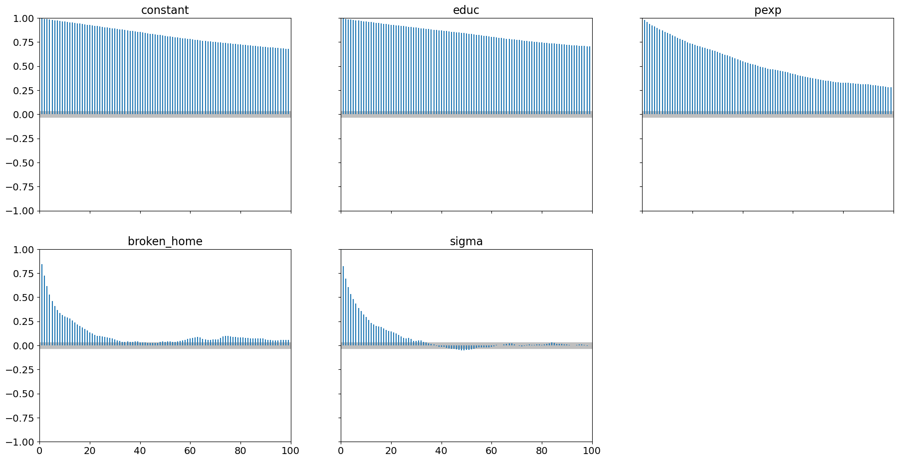
which shows very high level of autocorrelation particularly for educ and the model constant.

The accept rate is

accept = samples.sample_stats.accepted.mean().to_numpy()
print("Acceptance Rate: ", accept.round(3))

Acceptance Rate:  0.126

To obtain better results, we need to either

1. Increase sample size (and tuning), or

2. Choose a different step method

At this point in the course, our only option is to increase sampling and tuning:

with ols_model:
    step = pm.Metropolis()
    samples = pm.sample(10000, step=step, tune=10000, initvals=startvals, cores=2, chains=4,
                       return_inferencedata=True, progressbar=False)

Multiprocess sampling (4 chains in 2 jobs)

CompoundStep

>Metropolis: [constant]

>Metropolis: [educ]

>Metropolis: [pexp]

>Metropolis: [broken_home]

>Metropolis: [sigma]

Sampling 4 chains for 10_000 tune and 10_000 draw iterations (40_000 + 40_000 draws total) took 32 seconds.

The rhat statistic is larger than 1.01 for some parameters. This indicates problems during sampling. See https://arxiv.org/abs/1903.08008 for details

The effective sample size per chain is smaller than 100 for some parameters.  A higher number is needed for reliable rhat and ess computation. See https://arxiv.org/abs/1903.08008 for details

We get better, albeit not acceptable, convergence diagnostics:

pm.summary(samples)

	mean	sd	hdi_3%	hdi_97%	mcse_mean	mcse_sd	ess_bulk	ess_tail	r_hat
constant	0.662	0.124	0.432	0.900	0.015	0.010	73.0	156.0	1.05
educ	0.089	0.009	0.072	0.105	0.001	0.001	76.0	162.0	1.05
pexp	0.081	0.007	0.068	0.093	0.000	0.000	240.0	910.0	1.02
broken_home	-0.002	0.036	-0.069	0.067	0.001	0.000	4752.0	7001.0	1.00
sigma	0.433	0.009	0.415	0.451	0.000	0.000	7234.0	8344.0	1.00

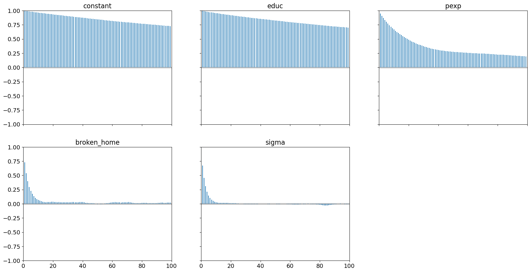
but we still have high levels of autocorrelation:

pm.plot_autocorr(samples, combined=True);

Our acceptance rate is also improved:

accept = samples.sample_stats.accepted.mean().to_numpy()
print("Acceptance Rate: ", accept.round(3))

Acceptance Rate:  0.317

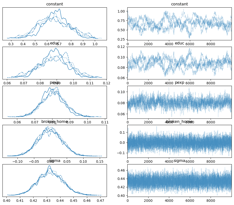
Here is the trace plot:

pm.plot_trace(samples);

Adding “policy relevant” measures to your model

It is possible to add policy relevant measures in your model and sample from those posteriors quite easily. For demonstration purposes, suppose we want to sample (1) the elasticity of education, and (2) the predicted wage. This is fairly straightforward but we need to redefine our PyMC model to include these items:

Recall that given the \(t^{th}\) sample for \(\beta_{kt}\) in our trace the elasticity in a semi-log model such as ours for individual \(i\) and variable \(k\) is

\[ E_{ikt} = b_{kt} x_{ik} \]

The average elasticity for variable \(k\) and and sample \(t\) is

\[ E_{kt} = \frac{\sum_{i=1}^{N} E_{ikt}}{N} \]

The expected elasticity of variable \(k\) as reflected by the underlying uncertainty in our posterior is

\[ E_{k} = \int E_{kt} p(\theta | x_i, h^0) d\theta \]

where \(\theta\) is the parameter vector and \(p(\theta|x_i, h^0)\) is our posterior and \(h^0\) are hyperparameters describing the priors.

We can approximate this integral using samples from the posterior. Since we have numerous samples for \(b_k\), we estimate the integral above using

\[ \hat{E}_k = \frac{\sum_{t=1}^T E_{kt}}{T} \]

where \(T\) is the number of samples in our trace.

To implement this in code, we will ask PyMC to store these calculations in our sampled chain which we can average to produce the desired measure. Note the use of pytensor.tensor for performing these calculations and the syntax pm.Deterministic tells pymc to include the calculated values in the trace.

import pytensor.tensor as tt

with pm.Model() as ols_model:
    ## priors
    b0 = pm.Normal('constant', mu=0., sigma=10.)
    b1 = pm.Normal('educ', mu=0., sigma=10.)
    b2 = pm.Normal('pexp', mu=0., sigma=10.)
    b3 = pm.Normal('broken_home', mu=0., sigma=10.)
    sigma = pm.Uniform('sigma', lower=.1, upper=10.)
 
    ## yhat (or the mean for each i's likelihood contrib)
    mu_i = b0 + b1 * tobias_koop.educ + b2 * tobias_koop.pexp +\
                b3 * tobias_koop.broken_home
        
    ## include some policy relevant measures in our samples
    # for predicted wage, note the model is in log wage units
    yhat = pm.Deterministic('wage_hat', tt.exp(mu_i))
    # this is E_{ikt} for a semi log model for each
    # sample from our posterior (N x T):
    elas_educ = b1 * tobias_koop.educ
    # note this will be calculated for **each** observation
    # for **each** sampled parameter vector.  What we want is
    # the average over all observations for each sampled parameter
    # vector (E_{kt}) whick we can calculate as 
    elas = pm.Deterministic('elas_educ', tt.mean(elas_educ, axis=-1))
 
    # likelihood
    like = pm.Normal('likelihood', mu=mu_i, sigma=sigma, 
                      observed=tobias_koop.ln_wage)

Now let’s sample from our posterior with these additional elements added in:

with ols_model:
    step = pm.Metropolis()
    samples = pm.sample(10000, step=step, tune=10000, initvals=startvals, cores=2, chains=4,
                       return_inferencedata=True, progressbar=False)

Multiprocess sampling (4 chains in 2 jobs)

CompoundStep

>Metropolis: [constant]

>Metropolis: [educ]

>Metropolis: [pexp]

>Metropolis: [broken_home]

>Metropolis: [sigma]

Sampling 4 chains for 10_000 tune and 10_000 draw iterations (40_000 + 40_000 draws total) took 33 seconds.

The rhat statistic is larger than 1.01 for some parameters. This indicates problems during sampling. See https://arxiv.org/abs/1903.08008 for details

The effective sample size per chain is smaller than 100 for some parameters.  A higher number is needed for reliable rhat and ess computation. See https://arxiv.org/abs/1903.08008 for details

Note

On some computers, this may not run due to memory limitations or could take a long time to run. If it fails to run on your machine, lower 10000 to some smaller value.

If we examine the samples object, note we have additional items:

samples.posterior

<xarray.Dataset>
Dimensions:         (chain: 4, draw: 10000, wage_hat_dim_0: 1034)
Coordinates:
  * chain           (chain) int64 0 1 2 3
  * draw            (draw) int64 0 1 2 3 4 5 6 ... 9994 9995 9996 9997 9998 9999
  * wage_hat_dim_0  (wage_hat_dim_0) int64 0 1 2 3 4 ... 1030 1031 1032 1033
Data variables:
    constant        (chain, draw) float64 0.7862 0.7862 0.7919 ... 0.7091 0.7022
    educ            (chain, draw) float64 0.08177 0.08177 ... 0.08651 0.08651
    pexp            (chain, draw) float64 0.07368 0.07368 ... 0.07455 0.07455
    broken_home     (chain, draw) float64 -0.05324 -0.05324 ... 0.04271 0.04271
    sigma           (chain, draw) float64 0.4054 0.4526 0.4353 ... 0.4195 0.4195
    wage_hat        (chain, draw, wage_hat_dim_0) float64 6.433 10.05 ... 7.409
    elas_educ       (chain, draw) float64 1.004 1.004 1.004 ... 1.062 1.062
Attributes:
    created_at:                 2024-01-12T10:54:02.394867
    arviz_version:              0.17.0
    inference_library:          pymc
    inference_library_version:  5.10.3
    sampling_time:              33.444486141204834
    tuning_steps:               10000

xarray.Dataset

• Dimensions:
  • chain: 4
  • draw: 10000
  • wage_hat_dim_0: 1034
• Coordinates: (3)
  • chain
    (chain)
    int64
    0 1 2 3

    array([0, 1, 2, 3])

  • draw
    (draw)
    int64
    0 1 2 3 4 ... 9996 9997 9998 9999

    array([   0,    1,    2, ..., 9997, 9998, 9999])

  • wage_hat_dim_0
    (wage_hat_dim_0)
    int64
    0 1 2 3 4 ... 1030 1031 1032 1033

    array([   0,    1,    2, ..., 1031, 1032, 1033])

• Data variables: (7)
  • constant
    (chain, draw)
    float64
    0.7862 0.7862 ... 0.7091 0.7022

    array([[0.78619073, 0.78619073, 0.79190343, ..., 0.49213354, 0.49213354,
            0.49213354],
           [0.89174926, 0.89174926, 0.89174926, ..., 0.59716091, 0.59716091,
            0.59716091],
           [0.75371312, 0.75371312, 0.75371312, ..., 0.68077152, 0.68077152,
            0.68077152],
           [0.70098131, 0.70098131, 0.71164194, ..., 0.71790865, 0.70909475,
            0.70224192]])

  • educ
    (chain, draw)
    float64
    0.08177 0.08177 ... 0.08651 0.08651

    array([[0.08176598, 0.08176598, 0.08176598, ..., 0.10214466, 0.10214466,
            0.10214466],
           [0.07172026, 0.07172026, 0.07172026, ..., 0.09152582, 0.09152582,
            0.09152582],
           [0.08124353, 0.08124353, 0.08124353, ..., 0.08925127, 0.08616911,
            0.08616911],
           [0.08452686, 0.08452686, 0.08528269, ..., 0.0865107 , 0.0865107 ,
            0.0865107 ]])

  • pexp
    (chain, draw)
    float64
    0.07368 0.07368 ... 0.07455 0.07455

    array([[0.07367943, 0.07367943, 0.07367943, ..., 0.07996503, 0.08147606,
            0.08539553],
           [0.07184395, 0.07184395, 0.07184395, ..., 0.0841209 , 0.0841209 ,
            0.0841209 ],
           [0.08023196, 0.08023196, 0.07605925, ..., 0.07980358, 0.08046118,
            0.08046118],
           [0.08041613, 0.08041613, 0.08041613, ..., 0.07454573, 0.07454573,
            0.07454573]])

  • broken_home
    (chain, draw)
    float64
    -0.05324 -0.05324 ... 0.04271

    array([[-0.05324338, -0.05324338, -0.05324338, ..., -0.01352026,
            -0.03455634, -0.03455634],
           [ 0.03860975,  0.03860975,  0.03860975, ...,  0.02709529,
             0.02709529,  0.02709529],
           [ 0.04085227,  0.04085227,  0.06745471, ...,  0.00110486,
             0.00110486,  0.00110486],
           [ 0.01724318,  0.01724318,  0.01724318, ...,  0.04270527,
             0.04270527,  0.04270527]])

  • sigma
    (chain, draw)
    float64
    0.4054 0.4526 ... 0.4195 0.4195

    array([[0.40539371, 0.45255652, 0.43533471, ..., 0.44179641, 0.44989939,
            0.40560546],
           [0.42394909, 0.44219523, 0.44219523, ..., 0.43377969, 0.43377969,
            0.43377969],
           [0.42869379, 0.42869379, 0.42869379, ..., 0.42647465, 0.42647465,
            0.42647465],
           [0.4338446 , 0.4338446 , 0.4338446 , ..., 0.41947776, 0.41947776,
            0.41947776]])

  • wage_hat
    (chain, draw, wage_hat_dim_0)
    float64
    6.433 10.05 10.86 ... 7.128 7.409

    array([[[ 6.43336669, 10.04824684, 10.86276134, ...,  7.9906598 ,
              7.30399019,  7.67401979],
            [ 6.43336669, 10.04824684, 10.86276134, ...,  7.9906598 ,
              7.30399019,  7.67401979],
            [ 6.47022378, 10.10581378, 10.92499467, ...,  8.03643871,
              7.34583514,  7.71798466],
            ...,
            [ 6.45128454, 10.42454957, 11.54455738, ...,  8.02120645,
              7.0834746 ,  7.17921962],
            [ 6.33611143, 10.48774764, 11.44171933, ...,  8.0454837 ,
              7.11565754,  7.2555588 ],
            [ 6.38597495, 10.6534688 , 11.80616665, ...,  8.10879953,
              7.19982011,  7.45738016]],
    
           [[ 6.92189791,  9.53461549, 11.44409556, ...,  7.68692447,
              7.15580698,  7.6916798 ],
            [ 6.92189791,  9.53461549, 11.44409556, ...,  7.68692447,
              7.15580698,  7.6916798 ],
            [ 6.92189791,  9.53461549, 11.44409556, ...,  7.68692447,
              7.15580698,  7.6916798 ],
    ...
            [ 6.76998466, 10.3683194 , 11.94809172, ...,  8.08407851,
              7.32429968,  7.71107836],
            [ 6.5327505 ,  9.92595349, 11.53936492, ...,  7.75285707,
              7.07229035,  7.53472057],
            [ 6.5327505 ,  9.92595349, 11.53936492, ...,  7.75285707,
              7.07229035,  7.53472057]],
    
           [[ 6.64177343,  9.88035702, 11.70952511, ...,  7.73062365,
              7.0748904 ,  7.57335291],
            [ 6.64177343,  9.88035702, 11.70952511, ...,  7.73062365,
              7.0748904 ,  7.57335291],
            [ 6.77412158, 10.10011543, 11.95188674, ...,  7.89659699,
              7.21586912,  7.70676927],
            ...,
            [ 7.01347795, 10.11229491, 11.96061061, ...,  7.98967308,
              7.24038357,  7.52570899],
            [ 6.95193351, 10.02355784, 11.85565427, ...,  7.91956238,
              7.176848  ,  7.45966964],
            [ 6.90445592,  9.95510287, 11.77468716, ...,  7.86547645,
              7.12783438,  7.40872451]]])

  • elas_educ
    (chain, draw)
    float64
    1.004 1.004 1.004 ... 1.062 1.062

    array([[1.00364975, 1.00364975, 1.00364975, ..., 1.25379113, 1.25379113,
            1.25379113],
           [0.88034189, 0.88034189, 0.88034189, ..., 1.12344842, 1.12344842,
            1.12344842],
           [0.99723682, 0.99723682, 0.99723682, ..., 1.09552918, 1.05769668,
            1.05769668],
           [1.03753854, 1.03753854, 1.0468162 , ..., 1.0618895 , 1.0618895 ,
            1.0618895 ]])

• Indexes: (3)
  • chain
    PandasIndex

    PandasIndex(Index([0, 1, 2, 3], dtype='int64', name='chain'))

  • draw
    PandasIndex

    PandasIndex(Index([   0,    1,    2,    3,    4,    5,    6,    7,    8,    9,
           ...
           9990, 9991, 9992, 9993, 9994, 9995, 9996, 9997, 9998, 9999],
          dtype='int64', name='draw', length=10000))

  • wage_hat_dim_0
    PandasIndex

    PandasIndex(Index([   0,    1,    2,    3,    4,    5,    6,    7,    8,    9,
           ...
           1024, 1025, 1026, 1027, 1028, 1029, 1030, 1031, 1032, 1033],
          dtype='int64', name='wage_hat_dim_0', length=1034))

• Attributes: (6)

  created_at :

  2024-01-12T10:54:02.394867

  arviz_version :

  0.17.0

  inference_library :

  pymc

  inference_library_version :

  5.10.3

  sampling_time :

  33.444486141204834

  tuning_steps :

  10000

In particular, note that we have a new dimension (or coordinate) in our chain, wage_hat_dim_0 which tracks observations in our data. Note, predicted wage is a large matrix:

samples.posterior.wage_hat.to_numpy().shape

(4, 10000, 1034)

Since we only have one elasticity measure per sampled parameter vector, it is

samples.posterior.elas_educ.to_numpy().shape

(4, 10000)

in a similar manner to our other parameters:

samples.posterior.constant.to_numpy().shape

(4, 10000)

In our calculations, we elected not to include individual-specific elasticities in our samples, hence there is no dimension over the observations in our data.

Analyzing the Trace

Summarizing the trace (and omitting our predicted wage) yields:

pm.summary(samples, var_names = ['constant', 'educ', 'pexp', 'broken_home', 'sigma', 'elas_educ'])

	mean	sd	hdi_3%	hdi_97%	mcse_mean	mcse_sd	ess_bulk	ess_tail	r_hat
constant	0.664	0.139	0.393	0.925	0.020	0.014	51.0	53.0	1.08
educ	0.088	0.010	0.070	0.107	0.001	0.001	52.0	59.0	1.07
pexp	0.081	0.007	0.069	0.093	0.001	0.000	169.0	751.0	1.02
broken_home	-0.003	0.036	-0.071	0.065	0.001	0.000	3076.0	7115.0	1.00
sigma	0.433	0.010	0.416	0.452	0.000	0.000	7719.0	8559.0	1.00
elas_educ	1.085	0.121	0.854	1.316	0.017	0.012	52.0	59.0	1.07

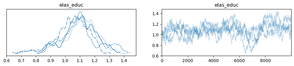
We can even see the marginal posterior for our elasticity estimate:

pm.plot_trace(samples, var_names = ['elas_educ']);

The predicted wage is included in the trace and is of dimension number of chains x number of samples x number of individuals. This is alot of information. To illustrate the information we have stored in our posterior let’s focus on only the first 50 individuals:

individs = [i for i in range(50)]
pm.plot_trace(samples.sel(wage_hat_dim_0 = individs), var_names=['wage_hat']);

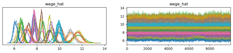
By storing these values in our trace, we can calculate policy relevant measures that immediately reflect the uncertainty of our parameter estimates since the distribution is being driven by the distribution of the posterior itself. This is evident in the posterior distributions of predicted wage for each individual.

Summary

This workbook has demonstrated how to use pymc for a linear regression model. We have examined some convergence criteria and see that we have to increase sample size quite alot to meet the Gelman-Rubin metric of r_hat \(\approx 1\). Even after increasing the number of samples by quite alot, the values above fail to completely satisfy this criteria for some of the parameters in our model.

In the next chapter we turn our attention to more modern step methods for achieving convergence with many fewer samples.